TLDR: This post accompanies The Developmental Landscape of In-Context Learning by Jesse Hoogland, George Wang, Matthew Farrugia-Roberts, Liam Carroll, Susan Wei and Daniel Murfet (2024), which shows that in-context learning emerges in discrete, interpretable developmental stages, and that these stages can be discovered in a model- and data-agnostic way by probing the local geometry of the loss landscape.
Four months ago, we shared a discussion here of a paper which studied stagewise development in the toy model of superposition of Elhage et al. using ideas from Singular Learning Theory (SLT). The purpose of this document is to accompany a follow-up paper by Jesse Hoogland, George Wang, Matthew Farrugia-Roberts, Liam Carroll, Susan Wei and Daniel Murfet, which has taken a closer look at stagewise development in transformers at significantly larger scale, including language models, using an evolved version of these techniques.
How does in-context learning emerge? In this paper, we looked at two different settings where in-context learning is known to emerge:
- Small attention-only language transformers, modeled after Olsson et al. (3m parameters).
- Transformers trained to perform linear regression in context, modeled after Raventos et al. (50k parameters).
Changing geometry reveals a hidden stagewise development. We use two different geometric probes to automatically discover different developmental stages:
- The local learning coefficient (LLC) of SLT, which measures the “basin broadness” (volume scaling ratio) of the loss landscape across the training trajectory.
- Essential dynamics (ED), which consists of applying principal component analysis to (a discrete proxy of) the model’s functional output across the training trajectory and analyzing the geometry of the resulting low-dimensional trajectory.
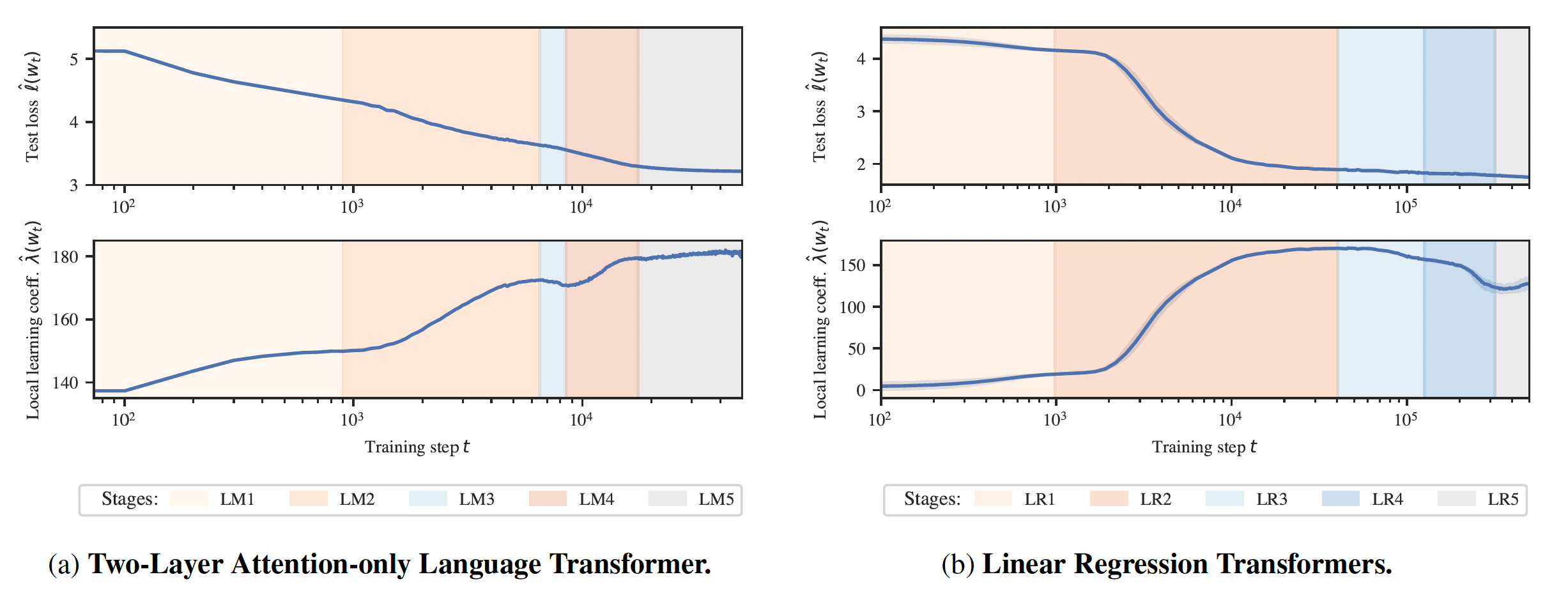
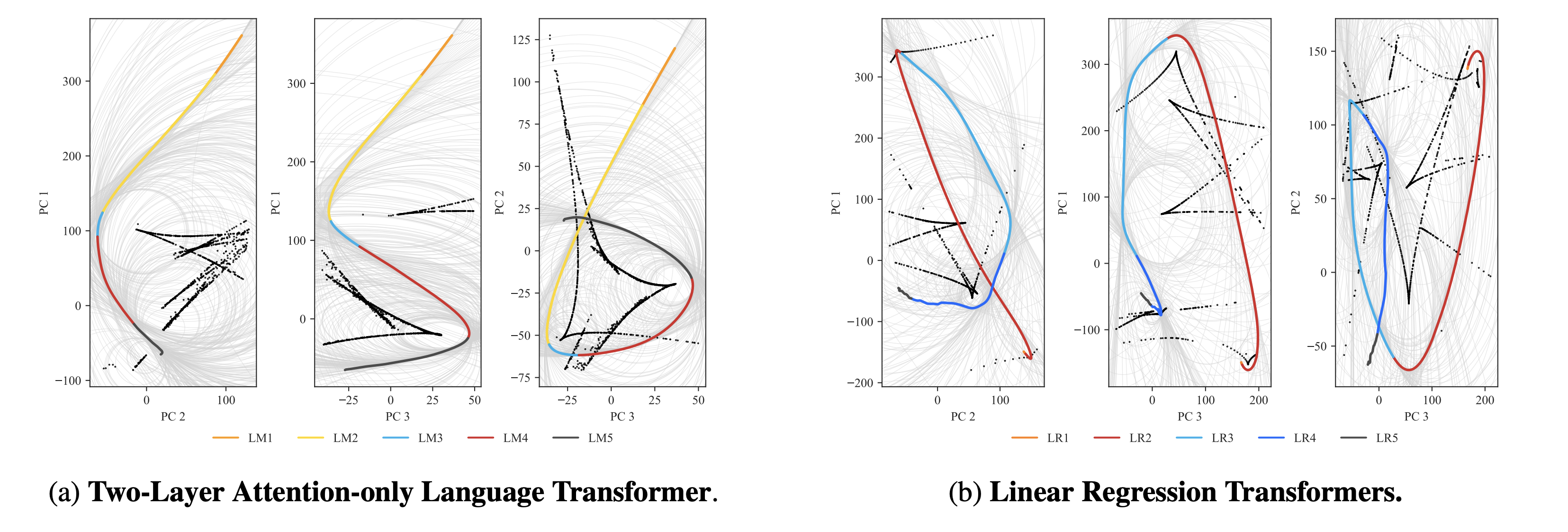
In both settings, these probes reveal that training is separated into distinct developmental stages, many of which are “hidden” from the loss (Figures 1 & 2).

**Figure 1: The development of 2-layer attention-only language transformers. **
Neural networks undergo stagewise development. This is often not visible in the loss (top left) but can be discovered by the local learning coefficient (bottom left) and essential dynamics (right three columns).

Figure 2: The development of linear-regression transformers. Plateaus in the LLC and particular kinds of turning points in ED identify developmental milestones that separate distinct stages.
Developmental stages are interpretable**.** Through a variety of hand-crafted behavioral and structural metrics, we find that these developmental stages can be interpreted.
The progression of the language model is characterized by the following sequence of stages:
- (LM1) Learning bigrams,
- (LM2) Learning various n-grams and incorporating positional information,
- (LM3) Beginning to form the first part of the induction circuit,
- (LM4) Finishing the formation of the induction circuit,
- (LM5) Final convergence.

Figure 3. Stage analysis of small language models. During stage LM1 the KL divergence between the model’s predictions and the empirical bigram distribution (the bigram score) approaches 0.3 nats (far left). During stage LM 2 loss on representative 3- and 4-grams relative to average loss increases dramatically (middle left). During stage LM 3 the previous-token score starts to increase for layer 1 heads 2 and 5 (middle). During stage LM 4 the prefix score starts to increase for layer 2 heads 7 and 8 (middle right) and the induction circuit ultimately finishes forming. This coincides with a drop in the ICL score (far right).

Figure 4: Developmental stages are interpretable**.** A language model learns bigrams, then n-grams, then it starts forming previous-token heads, then it completes the induction circuit, then it finally converges. Here you see changes in per-token loss: red means decrease, blue means increase.
The evolution of the linear regression model unfolds in a similar manner:
- (LR1) Learns to use the task prior (equivalent to learning bigrams),
- (LR2) Develops the ability to do in-context linear regression,
- (LR3-4) Two significant structural developments in the embedding and layer norms,
- (LR5) Final convergence.

Figure 5. Stage analysis of linear regression transformers. During stage LR1 the model learns to predict using the *task prior *\(\mathbf{x} \mapsto 0\) as shown by the average norm of predictions nearly disappearing (far left). During stage LR2 the model learns to perform in-context regression as demonstrated by the ICL score which measures loss on the last input minus loss on the input (middle left). During stage LR3 the unembedding “collapses” vanish and many of the LN weights go to zero (middle right). During stage LR4 the LN collapse extends to earlier layers (not pictured here) and the positional encoding collapses onto a low-rank subspace (far right).
Developmental interpretability is viable**.** The existence and interpretability of developmental stages in larger, more realistic transformers makes us substantially more confident in developmental interpretability as a viable research agenda. We expect that future generations of these techniques will go beyond detecting when circuits start/stop forming to detecting where they form, how they connect, and what they implement.
On Stagewise Development
Complex structures can arise from simple algorithms. When iterated across space and time, simple algorithms can produce structures of great complexity. One example is evolution by natural selection. Another is optimization of artificial neural networks by gradient descent. In both cases, the underlying logic — that simple algorithms operating at scale can produce highly complex structures — is so counterintuitive that it often elicits disbelief.
A second counterintuitive fact is that the changes produced by these iterative processes are not always distributed uniformly across time. Periods of relative stasis can be punctuated by bursts of rapid transformation. In the development of organisms within a single lifetime, there can be distinct stages characterized by qualitatively different modes of change, without any alteration to the underlying algorithm of iterative accumulation.
Biological systems develop in discrete stages. This phenomena of *stagewise development *is universal in biology (Gilbert & Barresi 2016), and it has been extensively studied by mathematicians (Freedman et al. 2021). The framework of dynamical systems theory views biological systems as complex networks of interacting components, with the behavior of the system determined by the collective dynamics of these interactions. In this context, distinct developmental stages are separated by bifurcations or critical points in the system’s dynamics.
What about neural networks? The same mathematics can be used to describe the training process of artificial neural networks, so it is not surprising to find that stagewise development occurs there as well. Indeed, this has been observed in simple neural networks for decades: Baldi and Hornik’s work in 1989 was very influential and McClelland and Rogers and collaborators studied similar phenomena in neuroscience and psychology. In recent years we have seen new and striking examples of stagewise development in transformers across a wide range of scales, as shown in Olsson et al. and other recent works.
Developmental Stages

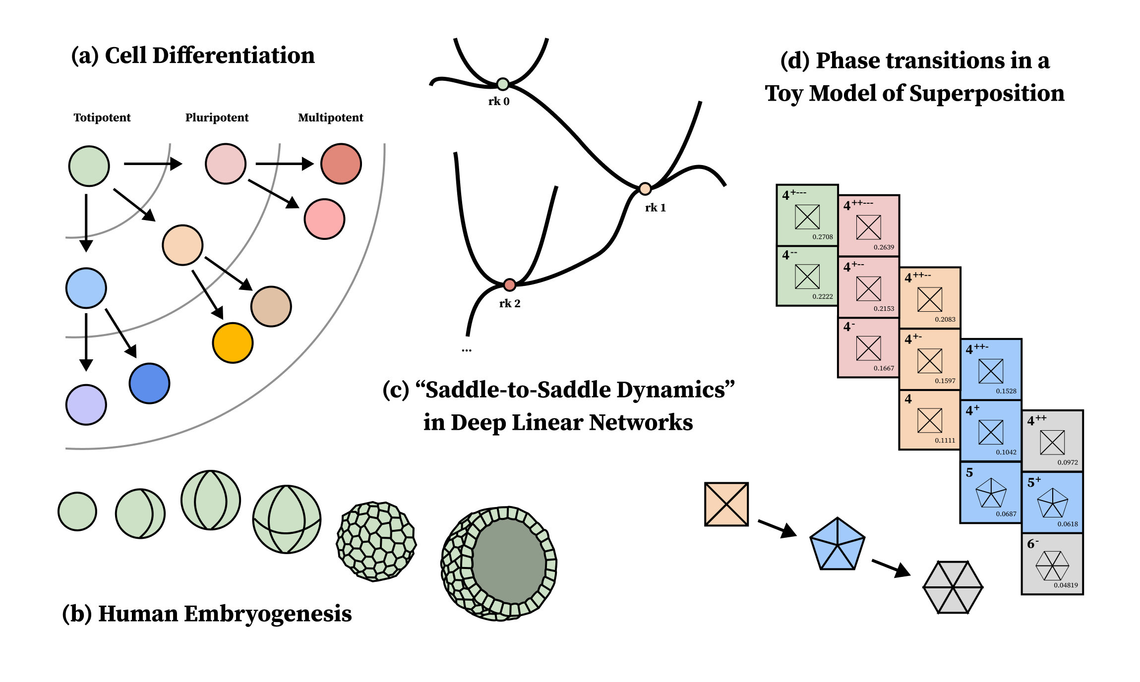
Figure 6: Examples of developmental stages.
Before attempting a general definition of what a stage of development is, let us consider some examples (figure 6):
- (a) Cell differentiation: Embryonic stem cells undergo a succession of several discrete “cell fate decision” events before reaching their final differentiated adult forms.
- (b) Human embryogenesis: Embryos go through fertilization, then cleavage, blastulation, implantation, and disc formation (which are divided into further substages).
- (c) “Saddle-to-saddle dynamics” in deep linear networks: With the right choice of initialization and scale separation, deep linear networks (that is, neural networks without the nonlinearities) undergo “saddle-to-saddle” dynamics.
- (d) Phase transitions in a toy model of superposition: As previously discussed, in a toy model of superposition, development consists of a series of phase transitions between different critical points, which can be enumerated.
We will define a stage of development to be a distinct period within a developmental process, characterized by specific patterns of change, organization, and functionality that are qualitatively different from those observed in other stages.
Developmental Milestones
Stages are often associated to the formation of particular structures and behaviors. The boundaries between stages, then, are particularly interesting targets for interpretability, as they represent a point at which some structure or behavior has finished forming.
We refer to these endpoints as developmental milestones.
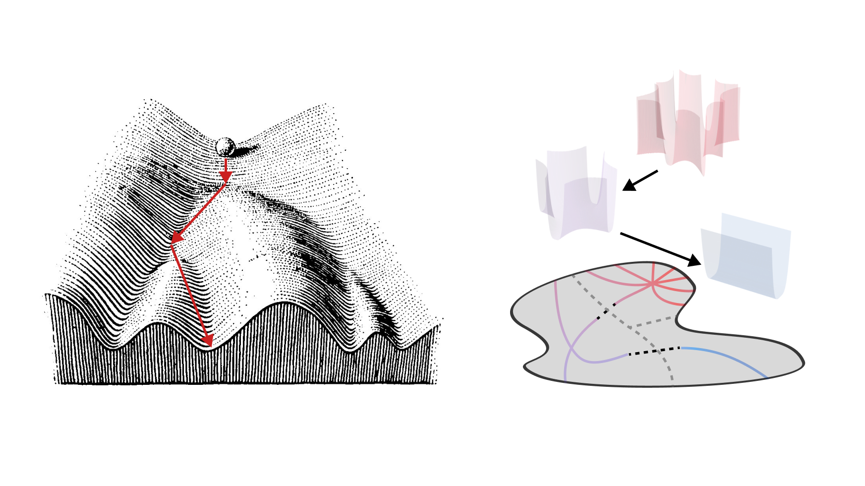
Milestones (sometimes) correspond to critical points. In the study of development through dynamical systems theory, it is common to associate the beginning and end of stages with critical points of a governing potential (Figure 7).
In the case of the toy model of superposition, we argued that this correspondence is exact: developmental milestones are governed by critical points of the loss landscape where \(\nabla L(w) = 0\). With this framing, developmental stages correspond to phase transitions, where the model’s trajectory \(w(t)\) through parameter space \(W\) over time \(t\) moves from one critical point of \(L(w)\) to another. At least in some theoretical treatments of deep linear networks (DLNs) this also seems to be the case: critical points of the population loss dominate the overall structure of learning.

Figure 7. Left: Waddington’s landscape. A basic idea in developmental biology is to think of development in terms of a succession of critical points. Right: The developmental landscape of neural networks. SLT predicts that neural network learning consists of a series of phase transitions between phases with different minimal loss and local learning coefficients \(\hat{\lambda}\).
What about larger models? In more realistic settings such as language models, training is not well-described as a sequence of paths connecting isolated critical points. This is clear from the fact that the loss does not pass through a series of plateaus, and the gradients never come close to vanishing. Nevertheless, there is plenty of prior evidence to suggest that the language of stages is also appropriate in the context of larger models. What, then, is the right notion of stage and milestone for such models?
Discovering Stages
We put forward two probes to study the geometry of the developmental trajectory: one for probing the loss landscape, the other for probing the trajectory through function space. Both probes reveal developmental stages and milestones in a data- and model-agnostic way.
The Local Learning Coefficient

Figure 8: Transformers undergo stagewise development. Development can be divided into discrete developmental stages that match SLT’s predictions of phase transitions. Many stages are “hidden” from loss (top) but can be discovered by tracking basin broadness (the LLC) over time (bottom).
SLT predicts phase transitions. Singular Learning Theory tells us that parameter space \(W\) can be coarse-grained into qualitatively distinct “phases” \({W_{\alpha} | \bigcup_\alpha W_\alpha= W}\) that are distinguished by their free energy:
\[F_n(W_{\alpha}) \approx n L_n(w_{\alpha}) + \lambda(w_{\alpha}) \log n \]
\(\)where \(n\) is the number of samples, \(w_{\alpha} \in W_\alpha\) is a particular critical point locally minimizing the loss \(L(w)\), and \(\lambda(w_{\alpha})\) is the local learning coefficient (LLC) associated to that point.
Bayesian learning can be recast as a variational problem of finding the phase that minimizes this free energy, which requires trading off the \(nL_n(w_\alpha)\) term against the \(\lambda(w_\alpha)\log n\) term. As \(n\) increases, this tradeoff can suddenly change to favor a different phase; this is a *Bayesian phase transition. *
With this theoretically-grounded framing, we can conceptualize the developmental trajectory as a pathway through different phases similar to the Waddington landscape analogy introduced earlier, where each phase has its own loss and LLC signature \((L_n(w_{\alpha}), \lambda_{\alpha})\). These two metrics thus become the most important to track, to a first approximation, in order to detect phase transitions (aka developmental stages).
Estimating the LLC. The LLC has many faces:
- Geometrically, \(\lambda(w_{\alpha})\) measures the volume scaling ratio of \(L(W_{\alpha})\) near \(w_\alpha\), heuristically, the “width” or “broadness” of the loss landscape in that phase.
- Structurally, \(\lambda(w_\alpha)\) measures a form of model complexity. While we don’t yet understand its algorithmic content in full, it is clear that this form of model complexity is more than just an “effective parameter count”.
- Statistically, \(\lambda(w_\alpha)\) can be estimated by measuring the (weighted-) average increase in loss in the neighborhood of \(w_\alpha\). For full details, see here.
Inferring milestones from the LLC. We perform LLC estimation at every model checkpoint \(w(t_1), \dots, w(t_T)\) to obtain the LLC over time, \(\hat{\lambda}(t):=\hat{\lambda}(w(t_j))\). Then, to identify milestones, we look for critical points where \(\)\(\partial \hat{\lambda}(t)/\partial t= 0\).
This relies on a slight sleight of hand: theoretically, LLC estimation assumes that you are measuring the LLC of a critical point of the loss where \(\nabla L(w)=0\). As mentioned above, this is not generally true for the training trajectories of realistic models. Hence it isn’t clear that tracking the LLC over training is justified.
Nonetheless critical points in the LLC curve do detect milestones, as confirmed by a large number of independent behavioral and structural metrics. Our working hypothesis is that the model is at a critical point for some subset of the data distribution, and the LLC curve is sensitive to this, however more theoretical work on this point is needed.
Interpreting the changes in LLC. If we have a \(\hat{\lambda}(t)\) curve which is relatively smooth with clearly distinguished stage boundaries, then each stage will either correspond to the LLC increasing or decreasing. We term these type A (orange hues) and type B transitions (blue hues), respectively.
We may think of a type A transition as coinciding with the formation of new structure (and acquisition of a new ability), such as the formation of an induction head, where model complexity increases as more information is being stored within it. Most of our identified stages are of this form and do indeed correspond to the onset of various abilities.
A type B transition can be loosely understood as a form of compression, where the model effectively discards information as it moves toward simpler algorithms that achieve the same performance. In the linear regression setting, stages LR3-4 exemplify type B transitions, characterized by a “collapse” in the layer norms and the embedding/unembedding. Independently of the LLC, these parts of the models seem to become simpler. The observed type B transition in LM3 remains mysterious.
…but we really care about function space. Measuring the geometry of the loss landscape is an important building block in the devinterp toolkit, since the loss landscape reflects important information about the internal structure of a model parameter. But ultimately, the we want to study how the model’s behavior changes across the course of its development, and the geometry of the loss is only a shadow of the geometry of function space.
Essential Dynamics
To understand how the behavior of a model \(f(x,w)\) changes over training, we need a way to probe the trajectory \(f(x,w(t))\) through function space 1. Unfortunately, function space is infinite dimensional. The natural solution, then, is to find a low-dimensional representation of the trajectory, and study the significant geometric features of that instead. This is the approach of essential dynamics.
Developmental trajectory in function space. Taking inspiration from biology and Olsson et al. 2022, we employed a technique termed (Functional) Essential Dynamics (ED). This is done by projecting high-dimensional model outputs of a given dataset onto a lower-dimensional space using Principal Component Analysis (PCA). With PCA we can obtain a “low-dimensional representation” of the model’s complicated trajectory, which in this case preserves about ~70% of the variance in the data. It turns out these simplified representations are actually highly structured, and in some cases they may even be directly interpretable.
Performing ED. Let \(f: \mathbb{R}^N \times W \to \mathbb{R}^M\) denote the transformer function \(f(x,w)\) for inputs \(x\)and parameters \(w\). Ideally we would like to study the functional trajectory \(f(x,w(t))\) directly and observe transitions in the computation of the network . But since we cannot measure the model’s output on every input \(x\), we are instead forced to measure a functional proxy over time.
Specifically, we fix an input dataset \(I = {x_i}{i=1}^n\) and track the transformer’s output on \(I\), resulting in a (flat) vector \({f(x_i, w(t))}{i=1}^n \in \mathbb{R}^{Mn}\). Stacking these column-vectors for each checkpoint time \(t_1, \dots, t_T\) gives us a \((Mn) \times T\) sized matrix, \(A\), to which we can apply PCA. This gives us a way to project each step of the model’s trajectory on to the top \(v=3\) principal components (i.e. the space spanned by the top \(v\) largest eigenvalues of \(A A^T \in \mathbb{R}^{Mn \times Mn}\)).
Then, we can plot the developmental trajectory projected onto combinations of principal components (the multi-colored trajectory in Figure 9).

Figure 9: Essential dynamics reveals that developmental trajectories are organized around a small set of circular orbits. At times, these orbits and their centers can themselves be interpreted. The trajectory is colored in by stages identified using LLC estimation. Osculating circles are plotted in gray in the background. Their centers, which form the evolute, are plotted as black dots. Cusps in this evolute identify turning points that potentially correspond to developmental milestones.
Inferring milestones from ED. The most salient feature in these developmental trajectories are the turning points. To locate these turning points, we plot osculating circles, that is, tangent circles whose radii are given by the inverse of the local curvature (visualized in gray in Figure 9). When the osculating circles are accentuated, it means that the trajectory locally behaves like it is in a circular orbit around a particular function. Formally, we look for cusps in the evolute, the set of centers of these osculating circles (black dots in Figure 9, see Rodriguez 2018).
Note that these cusps can be misleading. They may be an artifact of the projection and do not necessarily tell us anything interesting about the developmental trajectory. For example, a random walk like Brownian motion produces similar shaped curves 2. To classify a cusp as meaningful then, we require that it occurs at the same time and at the same PC coordinates across different projections. We call the underlying point in the functional proxy space that generates such a consistent cusp a form.
Interpreting the forms. Given a cusp with consistent PC coordinates across multiple projections, we can lift such a point up to the original functional proxy space to estimate the location of the form and interpret it. In the language modeling setting, we find two such forms, which correspond to the model learning word completion (that the next token should start with a space) and the induction mechanism (AB...[A]B).
Though the study of forms is still in its early days and requires many more sanity checks, we think that a future theory of forms may answer what the correct notion of developmental milestones is for realistic models — one that recovers the notion of milestones as critical points in simpler toy models.
Implications
The aim of developmental interpretability (“devinterp”) is to understand structure in terms of how it forms. Tracking changes over training provides a rich source of information for identifying when behaviors emerge, where the associated mechanisms establish themselves, and how those mechanisms relate to one another.
Our major takeaways from this paper were that:
- Developmental stages exist for more realistic models, which validates a major prediction of SLT.
- Developmental stages are interpretable, which validates developmental interpretability as a viable path towards interpretability.
- There is a path towards a better theory of developmental milestones, which was opened up via the theory of forms.
Over the next months, we will be focusing on scaling these techniques to larger models, developing new techniques that can pick up more fine-scale information about what is changing during these stages, and advancing the theory to open the way to later generations of tools. We now think this is actually going to work.
For more, read the paper.
Footnotes
-
Here the function space in question is the Hilbert space (L^2(X, q(x))), where (X) is the sample space and (q(x)) is the input distribution, with the usual inner product (\langle f(x), g(x)\rangle = \int f(x)g(x)dx). When we only have a finite set of samples (x_i \in X) drawn from (q(x)), the function space in question is the discrete counterpart with (\langle f, g\rangle = \sum_{i=1}^n f(x_i) g(x_i)). ↩
-
When the principal component scores (i.e. the result of the projections) are purely sinusoidal, these are known as Lissajous curves. ↩
Discussion
Join the conversation on LessWrong to discuss this post with the community.