TLDR; This is the second main post of Distilling Singular Learning Theory which is introduced in DSLT0. I synthesise why Watanabe’s free energy formula explains why neural networks have the capacity to generalise well, since different regions of the loss landscape have different accuracy-complexity tradeoffs. I also provide some simple intuitive examples that visually demonstrate why true parameters (i.e. optimally accurate parameters) are preferred according to the RLCT as\(n \to \infty\), and why non-true parameters can still be preferred at finite \(n\) if they have lower RLCT’s, due to the accuracy-complexity tradeoff. (The RLCT is introduced and explained in DSLT1).
It is an amazing fact that deep neural networks seem to have an inductive bias towards “simple” models, suggesting that they obey a kind of Occam’s Razor:
Plurality should not be posited without necessity.
or in modern parlance,
If two models of the world are similarly accurate, the simpler explanation should be preferred.
This allows them to achieve exceptionally low generalisation error despite classical statistics predictions that they should overfit data:
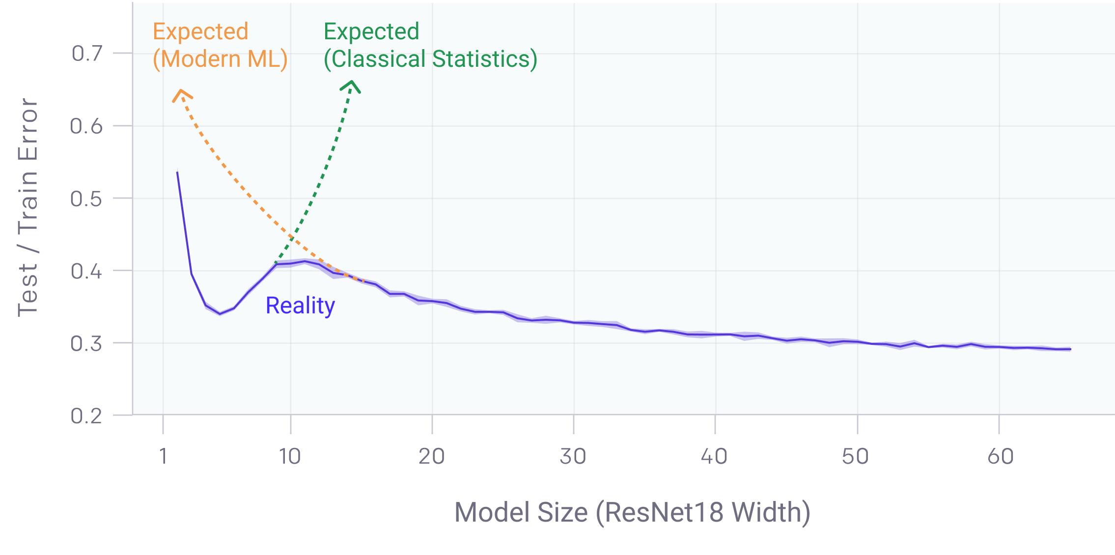
Neural networks seem to obey a kind of double descent where bigger is better, breaking classical statistics predictions.
(Source: OpenAI’s Double Descent blogpost).
This fact has come to be known as the generalisation problem and has been discussed at length in Zhang et. al 2017 (and a 2021 supplement), and in Bengio et al., amongst countless others.
Remarkably, Singular Learning Theory can help explain why neural networks, which are singular models, have the capacity to generalise so well.
The degeneracy of the Fisher information matrix is actually a feature of singular models, not a bug. This is because different regions of parameter space can have different complexities as measured by the RLCT \(\lambda\), unlike regular models where the complexity is fixed to the total number of parameters in the model \(d\). This is the implicit content of Watanabe’s profound free energy formula, called the Widely Applicable Bayesian Information Criterion (WBIC), which quantifies a precise asymptotic tradeoff between inaccuracy and complexity,
\[\mathrm{WBIC} = n \underbrace{ L_n(w^{(0)})}{\text{inaccuracy}} + \underbrace{\lambda }{\text{complexity}} \log n ,,\]
giving a mathematically rigorous realisation of Occam’s Razor, since \(\lambda \leq \frac{d}{2}\) in singular models.
In this post we will explore Watanabe’s free energy formula and provide an intuitive example of why the RLCT matters so much. If you are new to statistical learning theory, I would recommend jumping straight to the examples and their related animations to gain the intuition first, and then return to the theory afterwards.
The four key points to take away are:
- As \(n \to \infty\), true parameters with the best accuracy will always be preferred.
- As \(n \to \infty\), if two true parameters are equally accurate but have different RLCT’s, the parameter with the lower RLCT is preferred.
- For finite but large \(n\), non-true parameters can be preferred by the posterior because of an accuracy-complexity tradeoff as measured by the WBIC.
- Parameters with low inaccuracy and small RLCT’s \(\lambda\) have low generalisation error (in a Bayesian sense) since the Bayes generalisation error \(G_n\) is the “derivative” of the free energy, so
\[G_n = L_n(w^{(0)}) + \frac{\lambda}{n} + o\left( \frac{1}{n} \right) ,.\]
Information Criteria Help Avoid Underfitting and Overfitting
In the last post, we derived the asymptotic free energy \(F_n\) as \(n \to \infty\) for regular models, called the Bayesian Information Criterion (BIC):
\[\mathrm{BIC} = n L_n(w^{(0)}) + \frac{d}{2} \log n ,,\]
where \(n\) is the total number of datapoints in the dataset \(D_n\), the optimal loss is \(L_n(w^{(0)})\) where \(w^{(0)} \in W\) is a maximum likelihood estimate (i.e. \(w^{(0)} = \mathrm{argmin}_{W}(L(w))\)), and \(d\) is the total dimension of parameter space \(W \subseteq \mathbb{R}^d\).
As a statistical practitioner, given some dataset \(D_n\), your goal is to find a model that you hope will represent the truth from some candidate list. You only have access to the truth via your (training) dataset \(D_n\), but you also want to ensure that it generalises to data beyond the dataset. You can use the BIC to compare model candidates across a set of model classes that you can think to compare, since it captures a precise asymptotic tradeoff between inaccuracy \(L_n(w^{(0)})\) and complexity \(\frac{d}{2}\). Under this paradigm, we should choose the model that achieves the lowest BIC as it is the best option for avoiding both underfitting and overfitting the data. Let’s consider a simple example in action:
Example 1: Suppose we have \(n=61\) datapoints drawn from a quadratic with Gaussian noise, \(y = x^2 + \varepsilon\) where \(\varepsilon \sim \mathcal{N}(0,0.15^2)\)1, where \(x\) is drawn according to a uniform prior \(q(x) = \frac{1}{2} \mathbf{1}(x \in [-1,1])\). After looking at our scatterplot of data \(D_n\), we could try models across the following set of model classes:
| Name | \(d\) | Model |
|---|---|---|
| Linear | 2 | \(f_1(x,w) = w_1x+ w_0\) |
| Quadratic | 3 | \(f_2(x,w) = w_2x^2 + w_1x + w_0\) |
| Cubic | 4 | \(f_3(x,w) = w_3x^3 + w_2x^2 + w_1x + w_0\) |
| Degree 15 | 16 | \(f_{15}(x,w) = w_{15}x^{15} + w_{14} x^{14} + \dots + w_1x + w_0\) |
(The degree 15 model is an extremity just to illustrate a point.)
Within each model class, we can then perform ordinary least squares regression 2 to find the model fit \(w^{(0)}\) with optimal loss \(L_n(w^{(0)})\) (which, in the regression case, is simply the mean-squared-error plus a constant3). With the optimal loss of each model class in hand, we can then compare the \(\mathrm{BIC}\) over our set of candidates.
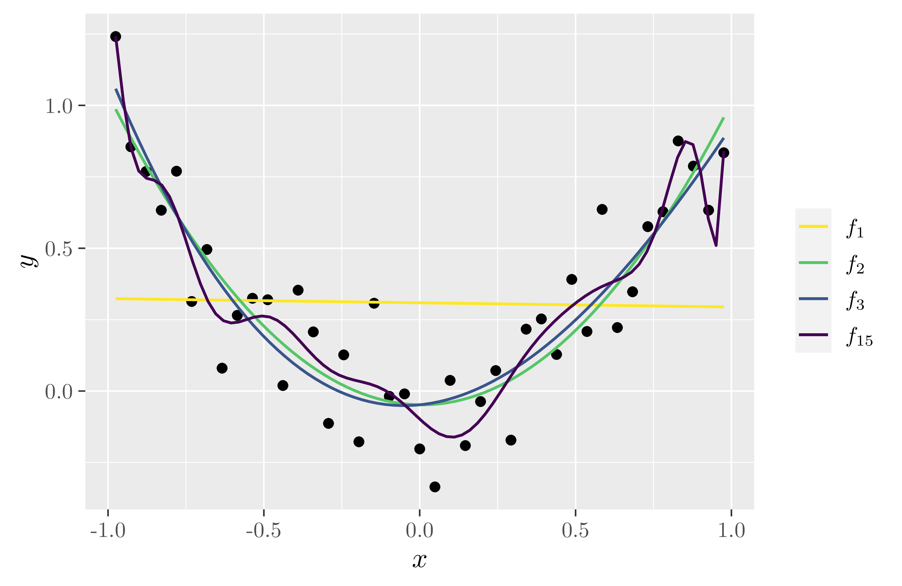
The optimal model fit to \(D_n\) for each model class, which vary in \(\mathrm{BIC}\) value.
| Model | \(L_n(w^{(0)})\) | \(d\) | \(\mathrm{BIC}\) |
|---|---|---|---|
| \(f_1(x, w)\) | 0.9668 | 1 | 63.09 |
| \(f_2(x, w)\) | 0.9283 | 2 | 62.80 |
| \(f_3(x, w)\) | 0.9280 | 3 | 64.83 |
| \(f_{15}(x, w)\) | 0.9243 | 15 | 87.22 |
As one expects, in a similar vein to the bias-variance tradeoff, there is a clear optimal (lowest) \(\mathrm{BIC}\). As the dimension increases, the accuracy gets better and better, but at the cost of the complexity of the model (and therefore, its generalisability4). The linear model is simple, but has high loss. The cubic has marginally lower loss, but at the expense of a complexity increase that isn’t worth it. The degree 15 polynomial has the lowest loss of them all, but is penalised heavily for its complexity (as it should be - it is clearly overfitting). The Goldilocks choice is unsurprisingly the quadratic model, \(f_2(x)\), because the tradeoff between accuracy and complexity is just right.
Other than the fact that the \(\mathrm{BIC}\) simply does not hold in the singular case, it also points us towards a limitation of regular models. Once you pick your model class to optimise, every point on the loss landscape has a fixed model complexity. If your goal is to minimise the \(\mathrm{BIC}\), you only have one choice: to find the single point that optimises the loss at the bottom of the well.
In fact, in our particular case, we can calculate the KL divergence 5 for the linear model \(f_2(x,w)\),
\[K(w_0, w_1) = \frac{1}{6} w_1^2 + \frac{1}{2} \left(w_0-\frac{1}{3} \right)^2 + \frac{2}{45},,\]
which we can see a plot of below.
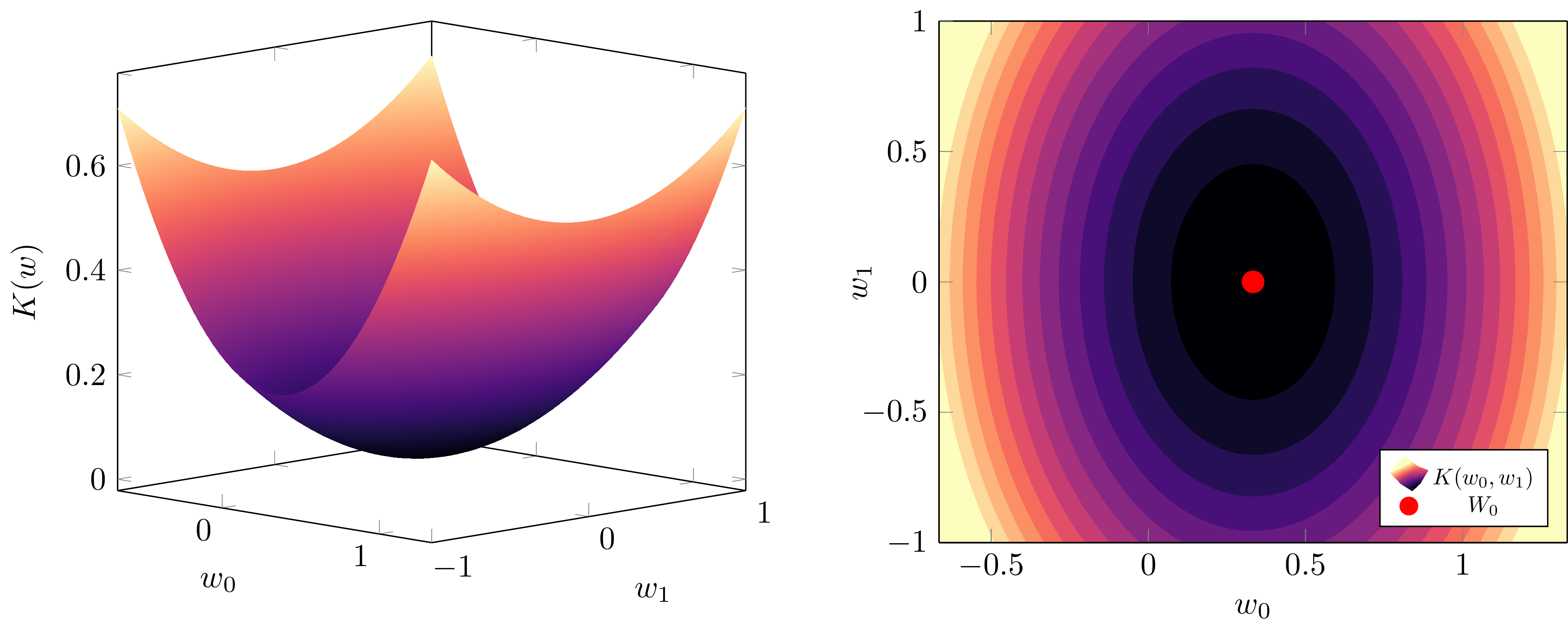
For a regular linear model with \(d=2\), parameters \(K(w)\) is just a paraboloid. Every point on its surface has the same complexity, \(\lambda = \frac{d}{2} = 1\), measuring the effective dimensionality.
In singular models, this all changes: within the same model class, different models \(w\) in parameter space \(W\) have different effective dimensionalities as measured by the RLCT \(\lambda\). The learning procedure does the work of the statistician for us, because the loss landscape contains information about both the accuracy and the complexity.
Watanabe’s Free Energy Formula for Singular Models
Free Energy, Generalisation and Model Selection
Fundamentally, we care about the free energy \(F_n = -\log Z_n\) because it is a measure of posterior concentration, and as we showed with the BIC calculation in DSLT1, it tells us something about the information geometry of the posterior. In particular, given a compact neighbourhood of parameter space \(\mathcal{W} \subseteq W\) we can define its local free energy
\[F_n(\mathcal{W}) = -\log \left( \int_{\mathcal{W}} \varphi(w) e^{-nL_n(w)} dw \right),,\]
providing a direct tool for comparing different regions of the posterior, and thus different models. Since there is a correspondence
\[\text{Small} ,, F_n(\mathcal{W}) \iff \text{Large posterior concentration} , \int_{\mathcal{W}} p(w|D_n)dw ,,\]
we say the posterior prefers a region \(\mathcal{W}\) when it has low free energy relative to other regions of \(W\).
But this isn’t the only reason to care about the free energy. In fact, it is explicitly related to generalisation, at least in the Bayesian sense.
In the frequentist framework that real-world deep learning takes place in (i.e. estimating a single parameter \(\hat{w}\) using SGD), we typically split our dataset \(D_n\) into a training set and a test set. We then say a model defined by \(\hat{w}\) generalises well when it has low loss on the test set - in other words, it performs well on data that it hasn’t seen before.
In the Bayesian paradigm, generalisation can be formulated according to a number of different estimation methods and quantities, depending on how you extract information from the posterior (e.g. you could estimate a maximum-likelihood parameter, a maximum a posterior estimate, or an average over samples from the posterior, etc.). Let’s focus on one for the moment that involves the Bayes predictive distribution given by
\[p(y|x,D_n) = \mathbb{E}w[p(y|x,w)] = \int{W} p(y|x,w) p(w|D_n) dw,,\]
which weights the probability of an output \(y\) given an input \(x\) according to the posterior measure. The Bayes generalisation loss is then given by
\[G_n = \mathbb{E}X[-\log p(y|x, D_n)] = -\iint{\mathbb{R}^{N+M}} q(y,x) \log p(y|x,D_n) dxdy ,.\]
Intuitively, it is the expected loss of the predictive distribution over all possible inputs \(x\) and outputs \(y\). It can be shown with relative ease 6 that the Bayes generalisation loss is equal to the average increase in free energy,
\[G_n = \mathbb{E}{X{n+1}}[F_{n+1}] - F_n ,.\]
In an informal-yet-conceptually-correct way, we can treat this difference as being the “derivative with respect to \(n\)” 7.
It follows immediately that the generalisation loss of a region \(\mathcal{W} \subseteq W\) is
\[G_n(\mathcal{W}) = \mathbb{E}{X{n+1}}[F_{n+1}(\mathcal{W})] - F_n(\mathcal{W}) ,.\]
Ergo, to understand the information contained in the posterior, and which regions contain models with low generalisation error, we want to calculate the free energy. In even modestly simple settings this integral is intractable, thus why we need to calculate its asymptotic form.
The Free Energy Formula for Singular Models
This subsection is a little bit more technical. If this overwhelms you, I recommend skipping ahead to the next subsection where I interpret the free energy formula.
As I explained in DSLT1, finding the asymptotic form of the free energy \(F_n\) as \(n \to \infty\) when \(I(w)\) is degenerate is hard, and depends of theorems of algebraic geometry and distribution theory. This formula has been refined over the course of many papers 8, adjusted and generalised with various hypotheses. Here we will focus on the form given in [Wat13], which also applies to the unrealisable case where the set of true parameters \(W_0\) may be empty. Thus we instead care about the set of optimal parameters
\[W_{\text{opt}} = \left{ w \in W ,|, L(w) = \min_{w’ \in W} L(w’) \right} ,,\]
and if \(W_0\) is non-empty, then \(W_0 = W_{\text{opt}}\). As it stands, the free energy formula in the unrealisable case depends on a hypothesis of *relatively finite variance *9.
Watanabe shows that the free energy of \(W\) asymptotically satisfies
\[F_n = n L_n(w^{(0)}) + \lambda \log n + U_n \sqrt{\frac{\lambda \log n}{2}} + O_p(1) \quad \text{as} , , n \to \infty.\]
where:
- \(n\) is the size of the dataset \(D_n\).
- \(w^{(0)} \in W_{\text{opt}}\) is a most singular optimal point of \(W\) (which we will explain below), which is in the interior of \(W\).
- \(\lambda \in \mathbb{Q}_{>0}\) is the global RLCT, associated to the most singular point \(w^{(0)}\).
- \({U_n}\) is a sequence of random variables that satisfies \(\mathbb{E}[U_n]=0\) and converges to a Gaussian random variable in law as \(n\to \infty\).
- \(O_p(1)\) denotes a sequence that is bounded in probability.
We will interpret the formula in a moment, but let me briefly clarify what it means to call \(w^{(0)}\) a “most singular point”, a notion is made precise in [Lin11, Proposition 3.9]. (See the below figure, too).
The gist is that every singularity \(w \in W_{\text{opt}}\) has an associated local RLCT \(\lambda_w\) defined by considering small neighbourhoods around the point. The global RLCT of \(W\) is defined to be the minimum over these optimal points, \(\lambda = \min_{w\in W_{\text{opt}}} {\lambda_w}\), and an optimal point \(w^{(0)} \in W_{\text{opt}}\) is a most singular point if \(\lambda_{w^{(0)}} = \lambda\) 10. Note also that the formula currently depends on an optimal parameter being in the interior of \(W\), so you can think of a most singular point as being a local minimum of \(K(w)\).
The Widely Applicable Bayesian Information Criterion
In the asymptotic limit as \(n \to \infty\), we can ignore the last two terms of the free energy formula and arrive at the Widely Applicable Bayesian Information Criterion (WBIC) across the full parameter space \(W\),
\[\mathrm{WBIC} = n L_n(w^{(0)}) + \lambda \log n ,.\]
Notice how the WBIC formula is the same as the BIC except that complexity is measured by \(\lambda\) instead of \(\frac{d}{2}\). But in DSLT1, we explained how
- In regular models \(\lambda = \frac{d}{2}\).
- In singular models \(\lambda \leq \frac{d}{2}\) in general.
Thus the WBIC is a generalisation of the BIC, containing the regular result as a special case.
Though the WBIC can be used to compare model classes like in the case of the BIC, its real power is what it tells us about the information geometry of the posterior within the same class of models. To this end, we can calculate the local free energy of a compact neighbourhood \(\mathcal{W} \subseteq W\)
\[F_n(\mathcal{W}) = n L_n(w^{(0)}{\mathcal{W}}) + \lambda{\mathcal{W}} \log n ,,\]
where \(w^{(0)}{\mathcal{W}} \in \mathcal{W}{\text{opt}}\) is the most singular optimal point in \(\mathcal{W}\) with associated RLCT \(\lambda_{\mathcal{W}}\).
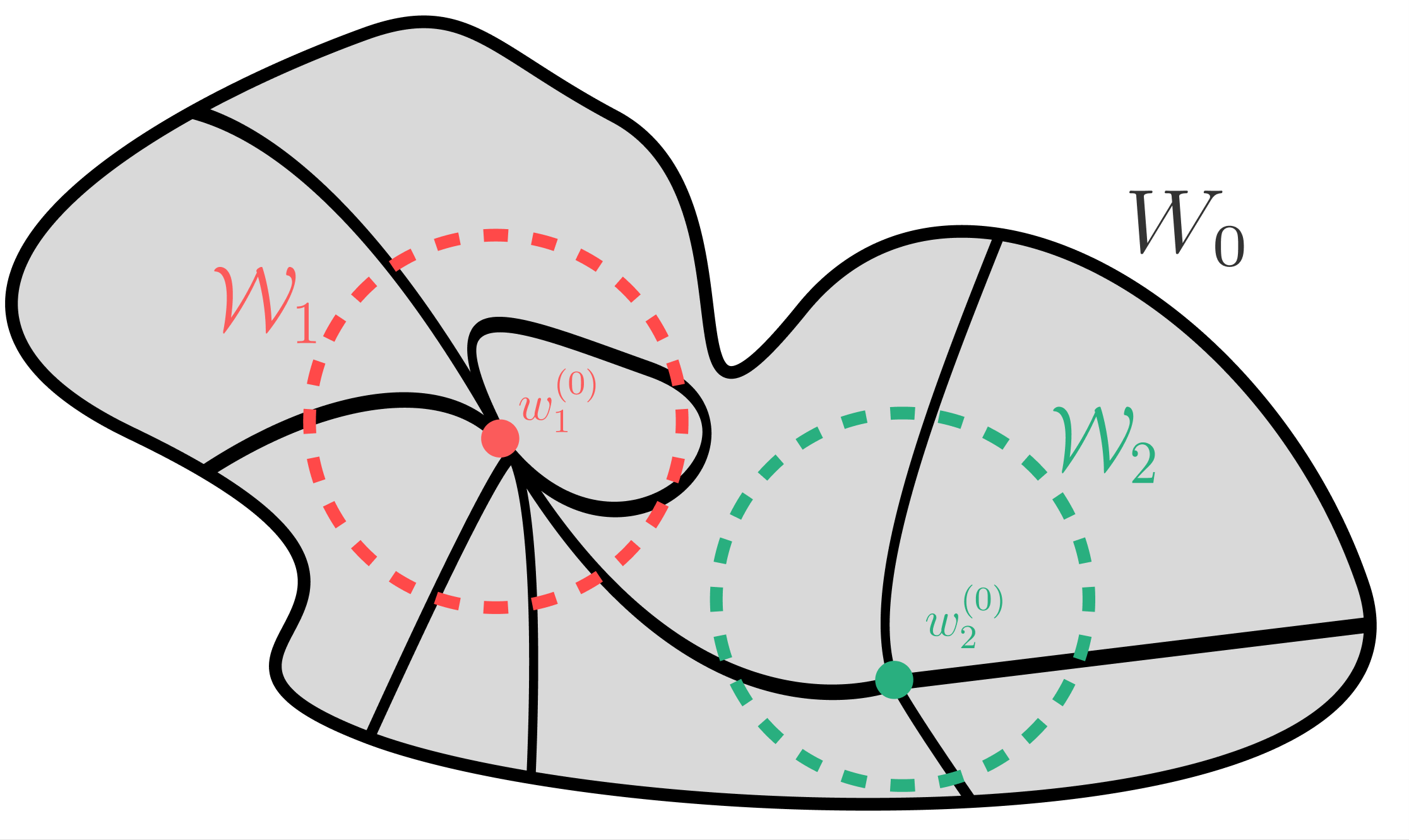
Here \(w^{(0)}_1\) is the most singular point of the local neighbourhood \(\mathcal{W}_1\), and \(w^{(0)}_2\) is the most singular point of \(\mathcal{W}_2\). Globally, \(w^{(0)}_1\) is the most singular point of all true parameters in \(W_0\) which means it dominates the total free energy \(F_n.\) In particular, \(F_n(\mathcal{W}_1) < F_n(\mathcal{W}_2)\) since \(\lambda_1<\lambda_2\).
(Thanks to Jesse for the figure template).
The Accuracy-Complexity Tradeoff
The WBIC shows that the free energy of a region \(\mathcal{W} \subseteq W\) is comprised of the accuracy and complexity (or, to the physicists, energy and entropy) of the most singular point in \(\mathcal{W}\)
\[F_n(\mathcal{W}) = n ,,\underbrace{ L_n(w^{(0)}{\mathcal{W}})}{\text{inaccuracy}} + \underbrace{\lambda_{\mathcal{W}} }_{\text{complexity}} \log n ,.\]
What makes this so profound is that in singular models, different regions \(\mathcal{W} \subset W\) can have different RLCT’s \(\lambda_{\mathcal{W}}\), each with a different tradeoff between accuracy and complexity, unlike the regular model case where every region has a fixed complexity:
\[\begin{aligned}\text{Regular models}&: F_n(\mathcal{W}) = n(\text{Inaccuracy}(\mathcal{W})) + \log n(\text{Constant Complexity}) \ \text{Singular models}&: F_n(\mathcal{W}) = n(\text{Inaccuracy}(\mathcal{W})) + \log n(\text{Complexity}(\mathcal{W})) \end{aligned}\]
So, the region in \(W\) that minimises the free energy has the best accuracy-complexity tradeoff. This is the sense in which singular models obey Occam’s Razor: if two regions are equally accurate, then they are preferred according to which is the simpler model.
Interpreting the terms in the free energy formula leads us to three main points:
- As \(n \to \infty\), regions \(\mathcal{W}\) containing optimal parameters \(w^{(0)} \in W_{\text{opt}}\) will always be preferred, since the inaccuracy is the leading order term.
- As \(n \to \infty\), if there are multiple regions \(\mathcal{W}_1\) and \(\mathcal{W}_2\) with equally optimal accuracy, then they are preferred according to their respective RLCT’s. Lower is better, so if \(\lambda_1<\lambda_2\) then \(\mathcal{W}_1\) is preferred by the posterior.
- For finite but large \(n\), regions that do not contain a globally optimal parameter can be preferred by the posterior because they can have a better tradeoff between accuracy and complexity.
Why Singular Models (Can) Generalise Well
Armed with our free energy formula, we can now understand why singular models have the capacity to generalise well.
Recall that the Bayes generalisation error can be expressed as the difference \(G_n = \mathbb{E}{X{n+1}}[F_{n+1}] - F_n\), which can be interpreted as the “derivative” of the free energy with respect to \(n\). Then since \(F_n = n L_n(w^{(0)}) + \lambda \log n\), Watanabe is able to prove in [Wat18, Chapter 8] that, asymptotically, the Bayes generalisation error is
\[\mathbb{E}[G_n] = L(w^{(0)}) + \frac{\lambda}{n} + o\left( \frac{1}{n} \right) ,.\]
In fact, he goes one step further by considering two other forms of generalisation, the leave-one-out-cross-validation-loss \(\mathrm{CV}\), and the WAIC (an empirically measurable form of the WBIC), and shows that asymptotically
\[\mathbb{E}[G_n] \approx \mathbb{E}[\text{CV}] \approx \mathbb{E}[\text{WAIC}] = L(w^{(0)}) + \frac{\lambda}{n} + o\left(\frac{1}{n} \right) ,.\]
Once again, we find that the RLCT \(\lambda\) plays a central role in the learning process. Most importantly, we have a correspondence:
\[\text{Optimal parameters with low RLCT} , \lambda \iff \text{Low generalisation error}.\]
On top of this, we can carry out the same analysis on our local \(F_n(\mathcal{W})\) to find that the local generalisation loss of \(\mathcal{W}\) is
\[\mathbb{E}[G_n(\mathcal{W})] = L(w^{(0)}{\mathcal{W}}) + \frac{\lambda{\mathcal{W}}}{n} ,.\]
Since the RLCT can differ region to region, this tells us that:
\[\text{In singular models, different regions have different generalisation error.}\]
All of this is to say: under any reasonable conception of Bayesian generalisation, the RLCT plays a central role in minimising generalisation loss, asymptotically. And since \(\lambda \leq \frac{d}{2}\) in singular models, the generalisation error of a singular model will always be better than that of a regular model with the same number of parameters. In DSLT3 we will show neural networks are singular, so:
This is why neural networks can generalise well!
…sort of. Don’t forget, we are in the Bayesian paradigm here, and it is not a given that Stochastic Gradient Descent (SGD) finds the same regions of parameter space that the Bayesian posterior says are “good”. We postulate that in some sense they are equivalent, and the work of Mingard et al. in Is SGD a Bayesian Sampler? Well, Almost. agrees with this postulate. But, formalising this relationship does remain a key open problem in conclusively applying SLT to modern deep learning with SGD and its variants.
From points to local neighbourhoods
For those with less background knowledge, there is an important conceptual shift we have made here that I want to elaborate on briefly.
In frequentist statistics we care about particular point estimates \(\hat{w}\) in parameter space \(W\). But in Bayesian statistics, we care about measurable regions \(\mathcal{W} \subset W\) of parameter space, and the probability to which the posterior assigns those regions. This is a powerful shift in perspective, and points towards why SLT is placed in a Bayesian paradigm: the observation the geometry of \(K(w)\) contains a lot more information than simple point estimates do lends itself naturally to Bayesian statistics.
But in modern deep learning, we only ever have access to a point estimate \(\hat{w}\) at the end of training via SGD. Sampling from the Bayesian posterior for large neural networks would not only be silly, but it would be, essentially, computationally impossible. So does this mean SLT has absolutely no applicability to modern deep learning?
Not at all. By studying the local geometry of the loss landscape \(K(w)\) - which is to say, arbitrarily small neighbourhoods \(\mathcal{W}\) of the posterior - we are able to analyse the set of points that are arbitrarily close to the singularities of \(K(w)\).
What Watanabe shows is that the singularities contained in these small neighbourhoods affect the geometry of the other points in the neighbourhood. If \(\mathcal{W}\) contains one true parameter \(w^{(0)} \in W_0\), the other points in \(\mathcal{W}\) may not be equal minima of \(K(w)\), but they are extremely close to being so. The same logic applies for the RLCT of a region: perhaps there is only one most singular point in \(\mathcal{W}\), but any nearby parameter within the small neighbourhood will define a model whose functional output is nearly identical to that of \(f(x,w^{(0)})\) which has a lower complexity.
In focusing only on points, we lose an extraordinary amount of information. So, we localise to neighbourhoods.
Intuitive Examples to Interpret the WBIC
It’s time we looked at a specific example to build intuition about what the WBIC is telling us.
I have constructed this toy example specifically to illustrate the main points here, and a lot of the details about the sub-leading terms in the free energy expansion are obfuscated, as well as the random fluctuations that make \(K_n(w)\) different to \(K(w)\). But, it is conceptually correct, and helps to illustrate the dominant features of the learning process as \(n \to \infty\). Don’t take it too literally, but do take it seriously.
We will start with some calculations, and then visualise what this means for the posterior as \(n \to \infty\).
Example 1: True parameters are preferred according to their RLCT
Let’s consider a one parameter model \(d=1\) with KL divergence defined by
\[K(w) = (w+1)^2(w-1)^4 ,,\]
on the region \(W = [-2,2]\) with uniform prior \(\varphi(w) =\frac{1}{4} \mathbf{1}(w \in W)\). There are two singularities in the set of true parameters,
\[W_0 = {-1, 1} ,,\]
which we will label as \(w^{(0)}_{-1}\) and \(w^{(0)}_1\) respectively. The Fisher information at true parameters is just the Hessian, which in the one dimensional case is simply the second derivative,
\[\begin{aligned} I(w^{(0)}) = J(w^{(0)}) = \frac{d^2 K}{d w^2} \Bigr|_{w=w^{(0)}} . \end{aligned}\]
\(\)An easy calculation shows
\[\frac{d^2 K}{dw^2} = 2(w-1)^2(15w^2+10w-1),,\]
\(\)meaning \(w_{-1}^{(0)}\) is a regular point and \(w_{1}^{(0)}\) is a singular point since
\[\frac{d^2 K}{dw^2}\Bigr|{w=-1} = 32,,\quad \text{whereas} \quad \frac{d^2 K}{dw^2}\Bigr|{w=1} = 0,,\]
meaning the Fisher information “matrix” (albeit it is one-dimensional) is degenerate at \(w_1^{(0)}\) but not at \(w_{-1}^{(0)}\). We thus expect the RLCT of \(w_{1}^{(0)}\) to be less than \(\frac{d}{2} = \frac{1}{2}.\)
Let \(B(w_0, \delta) = [w_0-\delta, w_0+\delta] \subset W\) denote a small neighbourhood of radius \(\delta>0\) centred at \(w_0\). To analyse the geometry of \(K(w)\) near the two singularities, we can define compact local regions
\[\mathcal{W}{-1} = B(w{-1}^{(0)}, \delta) \quad \text{and} \quad \mathcal{W}{1} = B(w{1}^{(0)}, \delta) ,.\]
By taking a Taylor expansion about each singularity, the leading order terms of \(K(w)\) in each region are
\[\begin{aligned} \mathcal{W}{-1}&: \quad K(w) \approx 16 (w+1)^2,, \ \text{and in} \quad \mathcal{W}{1}&: \quad K(w) \approx 4 (w-1)^4 ,,\end{aligned}\]
since \(\delta\) is very small. Recalling the definition of the RLCT from DSLT1, since \(K(w)\) is in normal crossing form we can read off the local RLCTs
\[\lambda_{-1} = \frac{1}{2} \quad \text{and} \quad \lambda_{1} = \frac{1}{4},,\]
meaning the effective dimensionalities associated to each singularity are \(2\lambda_{-1} = 1\) and \(2\lambda_{1}= \frac{1}{2}\) respectively.
Here’s the crux: since both singularities \(w_{-1}^{(0)}\) and \(w_{1}^{(0)}\) are true parameters, so \(K(w^{(0)}{-1}) = K(w^{(0)}{1})=0\), they both have the same accuracy \(S\) (a constant),
\[L(w_{-1}^{(0)}) = L(w_{1}^{(0)}) =S.\]
But, since the RLCT associated to \(\mathcal{W}{1}\) is smaller, \(\lambda{1} < \lambda_{-1}\), the free energy formula tells us that \(\mathcal{W}_{1}\) is preferred by the posterior since it has lower free energy,
\[F_n(\mathcal{W}{1}) < F_n(\mathcal{W}{-1}) ,,\]
and our generalisation formula tells us that \(\mathcal{W}_1\) will have lower expected Bayesian generalisation loss,
\[G_n(\mathcal{W}1) < G_n(\mathcal{W}{-1}) ,.\]
The simpler model is preferred, and has a lower generalisation loss, because it has a lower RLCT.
Notice here how our \(\delta\) was arbitrary. It doesn’t matter exactly what it is, because as long as it is small, \(K(w)\) will look like \(16(w+1)^2\) and \(4(w-1)^4\) in each respective region. Its geometry is dominated by these terms when very close to each singularity.
\(K(w)\) is like a potential well, where a lower RLCT means a flatter floor
We argued in the first post that the RLCT is the correct measure of “flatness” in the loss landscape. We can now see that with our own eyes by plotting \(K(w)\) in our above example:
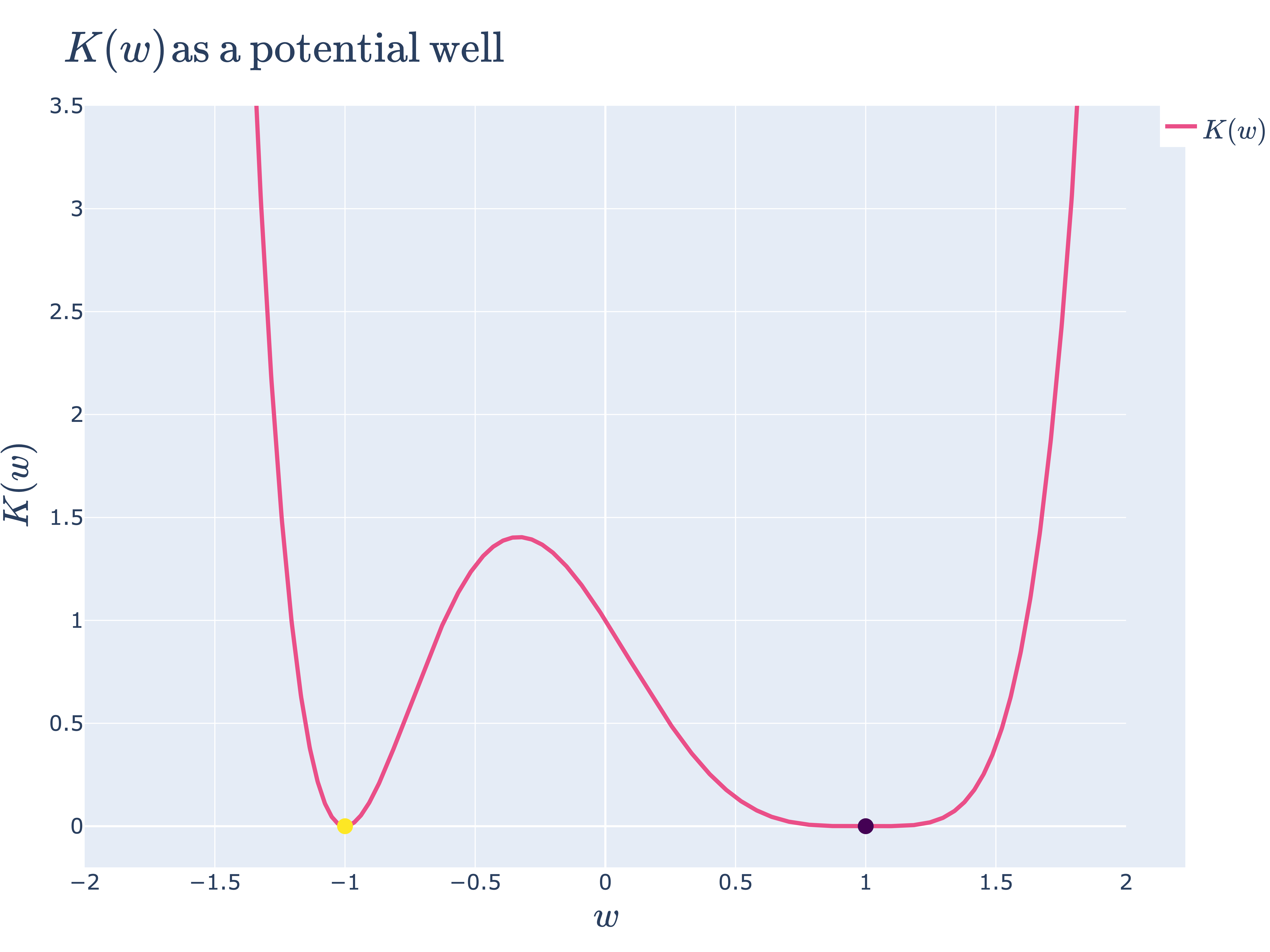
\(K(w) =(w+1)^2(w-1)^4\) is like a potential well. The particle is more likely to spend time in \(\mathcal{W}_1\) since it is flatter.
Looking at this plot, a good intuition to have is that the loss landscape \(K(w)\) is a potential well for some kinetic ball bouncing around, with its Hamiltonian given by \(H(w) \approx nK(w)\). The ball, with enough random kinetic energy, will explore both regions \(\mathcal{W}_{-1}\) and \(\mathcal{W}_1\), but it will spend more time in the latter since it is “flatter” 11.
Animation 1: The posterior concentrates on both true parameters as \(n \to \infty\), but it prefers the one with lower RLCT
For large \(n\), the empirical KL divergence is approximately equal to the KL divergence \(K_n(w) \approx K(w)\), and so normalising out by the constant \(S\), the posterior effectively only depends on \(K(w)\):
\[p(w|D_n) \approx \frac{\varphi(w) e^{-nK(w)}}{\int_{-2}^2 \varphi(w) e^{-nK(w)}dw} ,,\]
which is shown with some easy algebraic manipulations 12.
The free energy formula predicts that \(\mathcal{W}1\) is preferred because \(\lambda_1\) is smaller than \(\lambda{-1}\). So let’s look at how the posterior changes with \(n\):
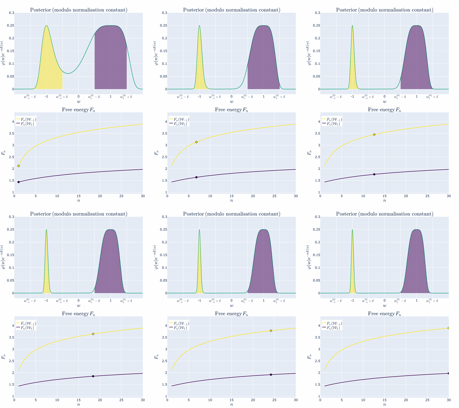
Both regions contain true parameters, but since \(\lambda_{1} < \lambda_{-1}\), the region \(\mathcal{W}_{1}\) is preferred by the posterior and thus has lower free energy.
As predicted, we visually see in the top posterior plot that the posterior concentration in \(\mathcal{W}{1}\) is greater than \(\mathcal{W}{-1}\) for all \(n\). The bottom plot backs this up precisely by showing that the free energy \(F_n(\mathcal{W}1)\) is always less than \(F_n(\mathcal{W}{-1})\). The RLCT clearly matters!
Note here that we have been able to numerically calculate the integrals \(Z_n(\mathcal{W}_{-1})\) and \(Z_n(\mathcal{W}_1)\), indicated by the shaded regions precisely, and not based on the free energy formula. This is because numerical integration is easy in low dimensions. In even modest dimensionality, these partition functions are notoriously difficult to compute, thus giving rise to the field of computational Bayesian statistics and algorithms like Markov Chain Monte Carlo. Our neural network experiments in DSLT4 require the MCMC approach.
Example 2: Non-true parameters can be preferred at finite \(n\) because of the accuracy-complexity tradeoff
Let’s alter our example ever so slightly to the case where \(\mathcal{W}1\) still has a lower RLCT, but it has marginally worse accuracy than \(\mathcal{W}{-1}\) and thus \(w_{1}^{(0)}\) is not a true parameter, but is an optimal parameter within \(\mathcal{W}_1\). We will set
\[\begin{aligned} &L(w^{(0)}{-1}) = S,, \ \text{and} \quad &L(w^{(0)}{1}) = S + C \end{aligned}\]
for some constant \(C>0\). Our KL divergence is then given by
\[K(w) = (w+1)^2 ((w-(1+h_C))^4 - k_C)\]
where \(h_C\) and \(k_C\) are constants chosen such that \(w^{(0)}_{1}=1\) is a local but not global minima of \(K(w)\), so \(K(1) = C\) and \(K’(1)=0\).
Then by the free energy formula 13,
\[\begin{aligned} F_n(\mathcal{W}{-1}) &= nS + \frac{1}{2} \log n,, \ F_n(\mathcal{W}{1}) &= n(S+C) + \frac{1}{4} \log n ,. \end{aligned}\]
We can visualise how this changes the loss landscape:
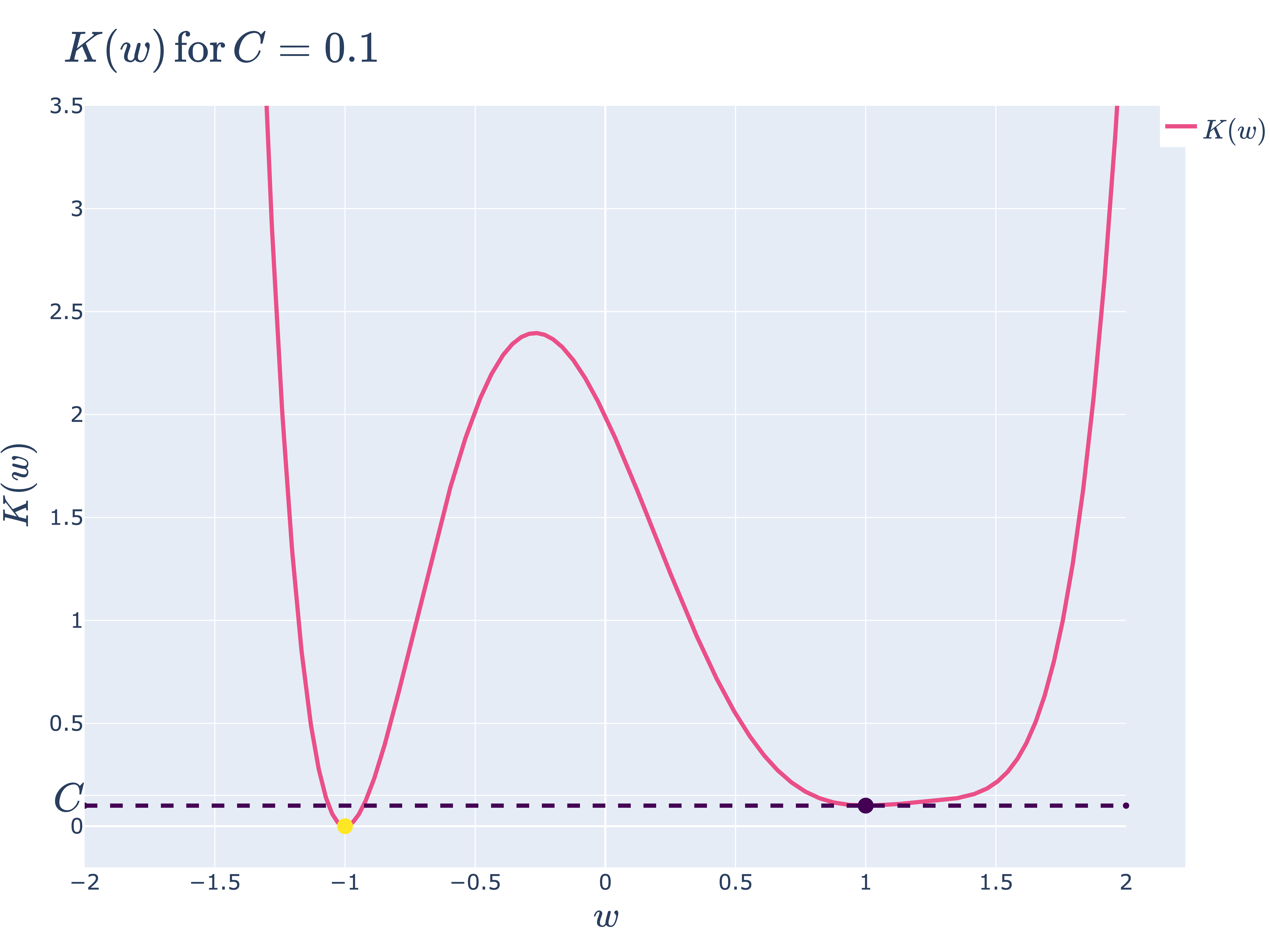
\(K(w)\) for \(C=0.1\), making \(w_1^{(0)}\) ever so slightly more inaccurate since \(K(w_1^{(0)})=C>0\).
Animation 2: At low \(n\) the simpler model is preferred, but as \(n \to \infty\), the true parameter is preferred\(\)
Let’s visualise how the posterior concentration changes with \(n\) for \(C=0.1\) and \(\delta = 0.5\) (yes, \(\delta\) is reasonably large here, but you want to be able to see this process, right?).
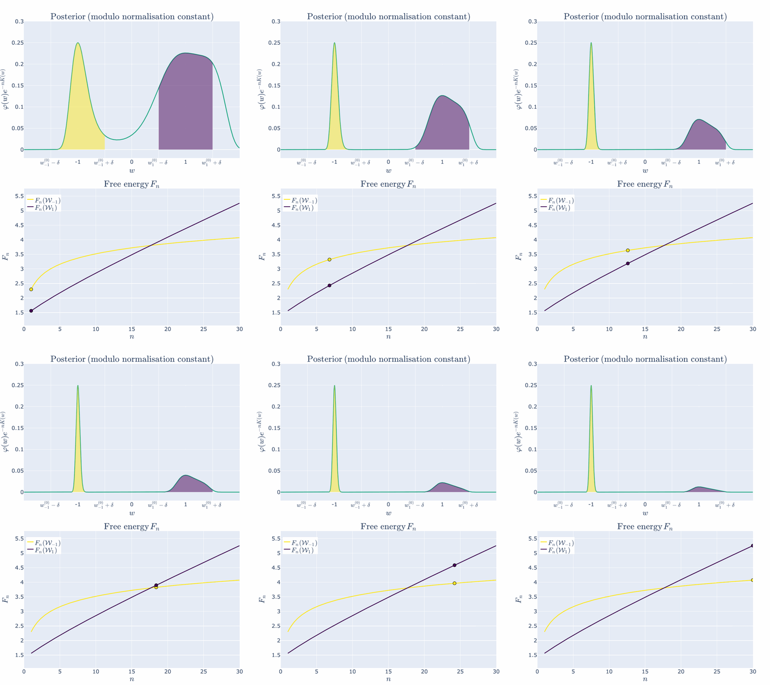
Here, \(w^{(0)}{-1}\) has the lower inaccuracy \(L(w^{(0)}{-1}) < L(w_{1}^{(0)})\), but \(w^{(0)}{1}\) has the lower complexity \(\lambda{1} < \lambda_{-1}\). The less accurate parameter can still be preferred at finite \(n\) because of the accuracy-complexity tradeoff, but as \(n \to \infty\), the more accurate parameter is preferred.
For the first few values of \(n\), the free energy is minimised by \(\mathcal{W}_{1}\) with its lower RLCT. But at about \(n \approx 17\) the inaccuracy of \(\mathcal{W}1\) has become too great to bare and the more accurate \(\mathcal{W}{-1}\) is preferred. After this point the free energy curves are monotonic - the more accurate model will be preferred for all \(n > 17\).
Asymptotic Analysis Requires Care
I know what you’re thinking: how come we could just approximate \(K(w)\) in each region? Don’t other curvature effects matter to the posterior density too? Like the prior, and those Taylor coefficients in \(K(w)\)? Wait, and don’t we care about \(K_n(w)\) instead of \(K(w)\)? Wait wait, \(K_n(w) = L_n(w) - S_n\), but we never have access to \(S_n\), so why would we care about \(K_n(w)\), let alone \(K(w)\)? This all seems far too contrived…
Yes, and no. Remember, the free energy formula gives us an asymptotic approximation of the posterior density has \(n \to \infty\). Thinking carefully about asymptotic approximations does require some care, particularly when one tries to convert these formulas into statements about finite \(n\) - after all, we can only ever train a model on a finite number of datapoints. But Watanabe’s free energy formula tells us what aspects of the geometry of \(K(w)\) affect the learning process as more data is collected. He is able to rigorously prove that the structure of singularities, as measured by the RLCT, are central to the long-term behaviour of model training. Yes, many other effects get thrown away in the \(O(1)\) term of the free energy formula, and the sequence \(U_n\) is also loaded with other random fluctuations, but Watanabe nonetheless shows what makes singular models so powerful.
Where are we going from here?
In this post, we have argued for the shift in perspective from points to local neighbourhoods (frequentist to Bayesian statistics), and then from local neighbourhoods to *singularities of *\(K(w)\) (classical learning theory to singular learning theory). We have gone from caring about an enormous parameter space \(W\), to only caring about certain singularities. Since singularities have different local geometry, and local neighbourhoods around them minimise the free energy, we have found our phases of statistical learning:
\[\text{Phases in learning} \iff \text{Local regions } \mathcal{W} \subset W \text{containing a singularity of interest } w^{(0)} ,.\]
We will explain this correspondence between phases and singularities in detail in DSLT4. Before that, though, in DSLT3 we are going to study the set of true parameters \(W_0\) of a particular toy model: two layer feedforward ReLU neural networks with two inputs and one output. In doing so, we will see how the singularities of \(K(w)\) in these models are identifiable with the different functionally equivalent symmetries of the neural network. With a full classification of \(W_0\) in hand, we will then look at some experiments on these toy models that provide tractable and precise illustrations of phase transitions in the posterior in these ReLU neural networks, which Watanabe’s free energy formula predicts.
References
[Wat09] S. Watanabe Algebraic Geometry and Statistical Learning Theory 2009
[Wat13] S. Watanabe A Widely Applicable Bayesian Information Criterion 2013
[Wat18] S. Watanabe Mathematical Theory of Bayesian Statistics 2018
[Lin11] S. Lin Algebraic Methods for Evaluating Integrals in Bayesian Statistics 2011
Footnotes
-
In other words, the true distribution is (q(y|x) = \mathcal{N}(x^2,1)). ↩︎ ↩
-
In other circumstances without a closed-form solution we can use an optimisation method like SGD. ↩
-
Precisely, [L_n(w) = \frac{1}{n} \sum_{i=1}^n \frac{1}{2} |y_i - f(x_i, w) |_M^2 + \frac{M}{2} \log 2\pi,,] where (M) is the dimension of the output (y \in \mathbb{R}^M). ↩︎ ↩
-
In the sense that if we kept drawing more data from the truth (q(y|x)), the error of (f_{15}(x)) would get worse and worse - it is overfitting data. ↩︎ ↩
-
Okay, so this is a bit of a white lie. If the model and truth are both defined by a regression model with equal variance (\sigma^2=1), then [K(w) = \frac{1}{2} \int_{\mathbb{R}^N} |f(x,w) - f(x,w_0)|^2_M q(x) dx ,.]I haven’t checked the case where the variances are different, but I believe it only requires a slight adjustment to this formula with a scaling factor somewhere. But this example nonetheless illustrates the point - (K(w)) is a paraboloid in regular models. ↩
-
Lemma 3.5 of my thesis. ↩︎ ↩
-
The reason this works is because of the asymptotics of (\log (n+1) - \log n). ↩
-
Originally, in [Wat09], Watanabe proves the formula for the realisable case where (w^{(0)} \in W_0) is a true parameter, meaning (K(w^{(0)})=0) and (L_n(w^{(0)})=S_n). ↩
-
[Wat18, Def 7, Chap 3] For a given pair (w_0 \in W_{\text{opt}}) and (w \in W), the log density ratio function is defined by [f(x,w_0,w) = \log \frac{p(y|x,w_0)}{p(x|w)} ,.]If there exists (c_0>0) such that for any arbitrary pair (w_0 \in W_{\text{opt}}) and (w \in W) [\mathbb{E}_X[f(X, w_0, w)] \geq c_0 \mathbb{E}_X[f(X, w_0, w)^2],,]then it is said that the log density ratio function (f(x,w_0,w)) has a relatively finite variance. ↩︎ ↩
-
And if it achieves the maximum multiplicity, but we will leave this vague to avoid more technical clutter. ↩
-
In fact, this analogy to statistical physics runs quite deep. Hamiltonian Monte Carlo, one of the main methods for sampling from a Bayesian posterior, is essentially just simulating a particle subject to a Gibbs distribution (e^{-H(w)}). There’s a reason we’ve been calling it the free “energy”, after all! ↩︎ ↩
-
Specifically, as (n \to \infty), the KL divergence converges, [L_n(w) - S_n = K_n(w) \to K(w) = L(w) - S ,.] Since (S) is a constant, we are able to write [\begin{aligned} p(w|D_n) &= \frac{\varphi(w) e^{-n L_n(w)}}{\int_W \varphi(w) e^{-n L_n(w)} dw} \ &\approx \frac{\varphi(w) e^{-n L(w)}}{\int_W \varphi(w) e^{-n L(w)} dw} \frac{e^{nS}}{e^{nS}} \ &= \frac{\varphi(w) e^{-n K(w)}}{\int_W \varphi(w) e^{-n K(w)} dw} ,. \end{aligned}]If one defines the posterior in terms of (K_n(w)), we call this the normalised posterior. ↩
-
For this pathological example, these formulas are certainly not an adequate approximation for the exact numerical free energy at low (n) - for one thing, they don’t even depend on the radius of the ball (\delta). However, writing the formulas like this does point us towards the conceptual idea, which is verified in the below animations. ↩
Discussion
Join the conversation on LessWrong to discuss this post with the community.