From Global to Local: A Scalable Benchmark for Local Posterior Sampling

Authors

Rohan Hitchcock

University of Melbourne

Jesse Hoogland

Timaeus

See Contributions

Publication Details

Published:

July 29, 2025

Access

Abstract

Degeneracy is an inherent feature of the loss landscape of neural networks, but it is not well understood how stochastic gradient MCMC (SGMCMC) algorithms interact with this degeneracy. In particular, current global convergence guarantees for common SGMCMC algorithms rely on assumptions which are likely incompatible with degenerate loss landscapes. In this paper, we argue that this gap requires a shift in focus from global to local posterior sampling, and, as a first step, we introduce a novel scalable benchmark for evaluating the local sampling performance of SGMCMC algorithms. We evaluate a number of common algorithms, and find that RMSProp-preconditioned SGLD is most effective at faithfully representing the local geometry of the posterior distribution. Although we lack theoretical guarantees about global sampler convergence, our empirical results show that we are able to extract non-trivial local information in models with up to O(100M) parameters.

Automated Conversion Notice

Warning: This paper was automatically converted from LaTeX. While we strive for accuracy, some formatting or mathematical expressions may not render perfectly. Please refer to the original ArXiv version for the authoritative document.

1 Introduction

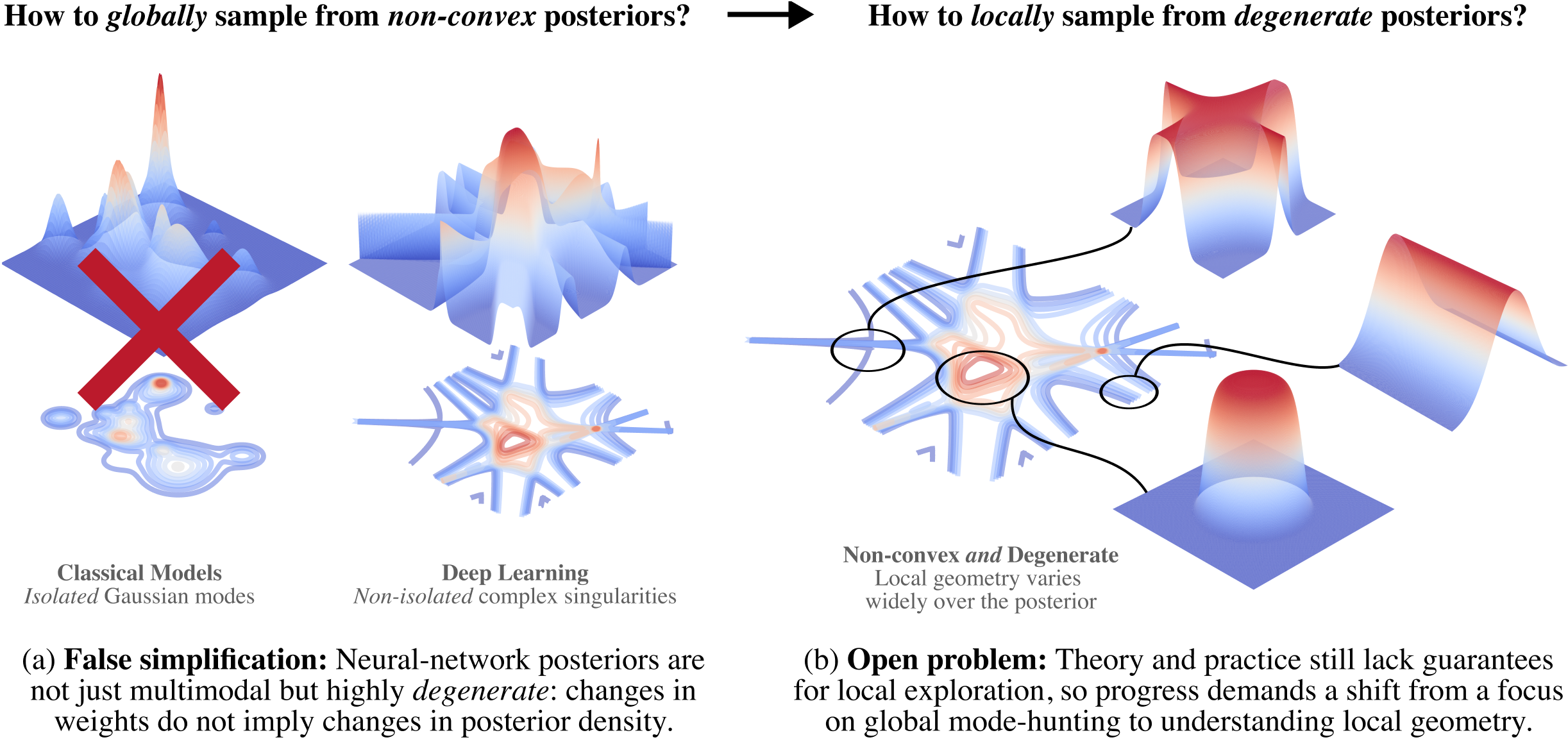
Neural networks have highly complex loss landscapes which are non-convex and have non-unique degenerate minima. When a neural network is used as the basis for a Bayesian statistical model, the complex geometry of the loss landscape makes sampling from the Bayesian posterior using Markov chain Monte Carlo (MCMC) algorithms difficult. Much of the research in this area has focused on whether MCMC algorithms can adequately explore the global geometry of the loss landscape by visiting sufficiently many minima. Comparatively little attention has been paid to whether MCMC algorithms adequately explore the local geometry near minima. Our focus is on Stochastic Gradient MCMC (SGMCMC) algorithms, such as Stochastic Gradient Langevin Dynamics (SGLD; Welling and Teh 2011), applied to large models like neural networks. For these models, the local geometry near critical points is highly complex and degenerate, so local sampling is a non-trivial problem.

In this paper we argue for a shift in focus from global to local posterior sampling for complex models like neural networks. Our main contributions are:

We identify open theoretical problems regarding the convergence of SGMCMC algorithms for posteriors with degenerate loss landscapes. We survey existing theoretical guarantees for the global convergence of SGMCMC algorithms, noting their common incompatibility with the degenerate loss landscapes characteristic of these models (e.g., deep linear networks). Additionally, we highlight some important negative results which suggest that global convergence may in fact not occur. Despite this, empirical results show that SGMCMC are able to extract non-trivial local information from the posterior; a phenomena which currently lacks theoretical explanation.
We introduce a novel, scalable benchmark for evaluating the local sampling performance of SGMCMC algorithms. Recognizing the challenge of obtaining theoretical convergence guarantees in degenerate loss landscapes, this benchmark assesses a sampler’s ability to capture known local geometric invariants related to volume scaling. Specifically, it leverages deep linear networks (DLNs), where a key invariant controlling volume scaling — the local learning coefficient (LLC; Lau et al., 2024) — can be computed analytically. This provides a ground-truth for local posterior geometry.
We evaluate common SGMCMC algorithms and find RMSProp-preconditioned SGLD (Li et al., 2016) to be the most effective at capturing local posterior features, scaling successfully up to models with O(100M) parameters. This offers practical guidance for researchers and practitioners. Importantly, our benchmark shows that although we lack theoretical guarantees about global sampling, SGMCMC samplers are able to extract non-trivial local information about the posterior distribution.

Refer to caption — Figure 1: **From global to local posterior sampling.** Left: Neural network posteriors are often erroneously simplified as isolated Gaussian modes. Middle: Neural network posterior distributions are highly degenerate, where parameter changes often don’t affect posterior density. Right: Local sampling must handle these degeneracies, which raises open theoretical and practical questions about the guarantees and effectiveness of local posterior exploration.

2 Background

In Section 2.1 we discuss existing theoretical results about the convergence of SGLD and related sampling algorithms. We highlight some important negative results from the literature, which suggest that global convergence of algorithms like SGLD are unlikely to occur in loss landscapes with degeneracy, and show that existing global convergence guarantees for SGLD rely on assumptions that likely do not hold for neural networks. In Section 2.2 we discuss applications and related work.

2.1 Problems with global sampling

We consider the problem of sampling from an absolutely continuous probability distribution $\pi(w)$ on $\mathbb{R}^{d}$ . In Bayesian statistics we often consider the tempered posterior distribution

\pi(w)\propto\varphi(w)\prod_{i=1}^{n}p(X_{i}|w)^{\beta}=\varphi(w)\exp(-n\beta L_{n}(w))

(2.1)

where $\{p(x|w)\}_{w\in\mathbb{R}^{d}}$ is a statistical model, $\varphi(w)$ the prior, $D_{n}=\{X_{1},\ldots,X_{n}\}$ a dataset drawn independently from some distribution $q(x)$ , $L_{n}(w)=\tfrac{-1}{n}\sum_{i=1}^{n}\log p(X_{i}|w)$ is the empirical negative log-likelihood, and $\beta>0$ is a fixed parameter called the inverse temperature. For any distribution, we can consider the overdamped Langevin diffusion; the stochastic differential equation

dW_{t}=\tfrac{1}{2}\nabla\log\pi(W_{t})dt+dB_{t}

(2.2)

where $B_{t}$ is standard Brownian motion. Under fairly mild assumptions on $\pi(w)$ (see Roberts and Tweedie, 1996, Theorem 2.1) (2.2) has well-behaved solutions and $\pi(w)$ is its stationary distribution. The idea of using the forward Euler-Maruyama discretisation of (2.2) to sample from $\pi(w)$ was first proposed by Parisi (1981) in what is now known as the Unadjusted Langevin Algorithm (ULA; also known as the Metropolis Langevin Algorithm), where for $t=0,1,\ldots$ we take

w_{t+1}=w_{t}+\Delta w_{t}\qquad\text{where}\qquad\Delta w_{t}=\tfrac{\epsilon}{2}\nabla\log\pi(w_{t})+\sqrt{\epsilon}\eta_{t}

(2.3)

where $\epsilon>0$ is the step size and $\eta_{0},\eta_{1},\ldots$ are a sequence of iid standard normal random vectors in $\mathbb{R}^{d}$ . Stochastic Gradient Langevin Dynamics (SGLD; Welling and Teh 2011) is obtained by replacing $\nabla\log\pi(w_{t})$ in (2.3) with a stochastic estimate $g(w_{t},U_{t})$ , where $U_{0},U_{1},\ldots$ are independent random variables. When $\pi(w)$ is given by (2.1), usually $g(w,U)$ is a mini-batch estimate of the log-likelihood gradient $g(w,U)=-\tfrac{n\beta}{m}\sum_{i=1}^{m}\nabla\log p(X_{u_{i}}|w)$ where $U=(u_{1},\ldots,u_{m})$ selects a random subset of the dataset $D_{n}$ .

Degeneracy can cause samplers to diverge.

Issues with ULA when $\log\pi(w)$ has degenerate critical points were first noted in Roberts and Tweedie (1996, Section 3.2), where they show that ULA will fail to converge to $\pi(w)$ for a certain class of distributions when $\log\pi(w)$ is a polynomial with degenerate critical points. Mattingly et al. (2002) relates the convergence of forward Euler-Mayuyama discretisations of stochastic differential equations (and hence the convergence of ULA) to a global Lipschitz condition on $\nabla\log\pi(w)$ , giving examples of distributions which do not satisfy the global Lipschitz condition for which ULA diverges at any step size. Hutzenthaler et al. (2011, Theorem 1) shows that if $\nabla\log\pi(w)$ grows any faster than linearly then ULA diverges. This is a strong negative result on the global convergence of ULA, since in models like deep linear networks, the presence of degenerate critical points causes super-linear growth away from these critical points.

The current theory makes strong assumptions about the loss landscape.

Given the above results, it is therefore no surprise that results showing that SGLD is well-behaved in a global sense rely either on global Lipschitz conditions on $\nabla\log\pi(w)$ , or on other conditions which control the growth of this gradient. Asymptotic and non-asymptotic global convergence properties of SGLD are studied in Teh et al. (2015); Vollmer et al. (2015). These results rely on the existence of a Lyaponov function $V:\mathbb{R}^{d}\to[1,\infty)$ with globally bounded second derivatives which satisfies

\|\nabla V(w)\|^{2}+\|\nabla\log\pi(w)\|^{2}\leq CV(w)\qquad\text{ for all }w\in\mathbb{R}^{d}

(2.4)

for some $C>0$ (see Teh et al., 2015, Assumption 4). The bounded second derivatives of $V(w)$ impose strong conditions on the growth of $\log\pi(w)$ and is incompatible with the deep linear network regression model described in Section 3.2. A more general approach to analysing the convergence of diffusion-based SGMCMC algorithms is described in Chen et al. (2015), though in the case of SGLD the necessary conditions for this method imply that (2.4) holds (see Chen et al., 2015, Appendix C).

Other results about the global convergence of SGLD and ULA rely on a global Lipschitz condition on $\nabla\log\pi(w)$ (also called $\alpha$ -smoothness), which supposes that there exists a constant $\alpha>0$ such that

\|\nabla\log\pi(w_{1})-\nabla\log\pi(w_{2})\|\leq\alpha\|w_{1}-w_{2}\|\qquad\text{ for all }w_{1},w_{2}\in\mathbb{R}^{d}.

(2.5)

This is a common assumption when studying SGLD in the context of stochastic optimization (Raginsky et al., 2017; Tzen et al., 2018; Xu et al., 2020; Zou et al., 2021; Zhang et al., 2022) and also in the study of forward Euler-Mayurmara discretisations of diffusion processes including ULA (Kushner, 1987; Borkar and Mitter, 1999; Durmus and Moulines, 2016; Brosse et al., 2018; Dalalyan and Karagulyan, 2019; Cheng et al., 2020). Other results rely on assumptions which preclude the possibility of divergence (Gelfand and Mitter, 1991; Higham et al., 2002).

Conditions which impose strong global conditions on the growth rate of $\nabla\log\pi(w)$ often do not hold when $\log\pi(w)$ has degenerate critical points. For concreteness, consider the example of an $M$ -layer deep linear network learning a regression task (full details are given in Section 3.2). Lemma 2.1 shows that assumptions (2.4) and (2.5) do not hold when $M>1$ , which is exactly the situation when $L_{n}(w)$ has degenerate critical points.

Lemma 2.1.

The negative log-likelihood function $L_{n}(w)$ for the deep linear network regression task described in Section 3.2 is a polynomial in $w$ of degree $2M$ with probability one, where $M$ is the number of layers of the network.

Proof.

We give a self-contained statement and proof in Appendix B.

All is not lost.

Despite the negative results discussed above and the lack of theoretical guarantees, Lau et al. (2024) shows empirically that SGLD can be used to obtain good local measurements of the geometry of $L_{n}(w)$ when $\pi(w)$ has the form in (2.1). This forms the basis of our benchmark in Section 3.2, and we show similar results for a variety of SGMCMC samplers in Section 4. In the absence of theoretical guarantees about sampler convergence, we can empirically verify that samplers can recover important geometric invariants of the log-likelihood. We emphasise that this empirical phenomena is unexplained by the global convergence results discussed above, and presents an open theoretical problem.

Some work proposes modifications to ULA or SGLD which aim to address potential convergence issues (Gelfand and Mitter, 1993; Lamba et al., 2006; Hutzenthaler et al., 2012; Sabanis, 2013; Sabanis and Zhang, 2019; Brosse et al., 2019). Finally, Zhang et al. (2018) is notable for its local analysis of SGLD, studying escape from and convergence to local minima in the context of stochastic optimization.

2.2 The need for local sampling

The shift toward local posterior sampling has immediate practical implications in areas such as interpretability and Bayesian deep learning.

Interpretability

SGMCMC algorithms play a central role in approaches to interpretability based on singular learning theory (SLT). SLT (see Watanabe, 2009, 2018) is a mathematical theory of Bayesian learning which properly accounts for degeneracy in the model’s log-likelihood function, and so is the correct Bayesian learning theory for neural networks (see Wei et al., 2022). It provides us with statistically relevant geometric invariants such as the local learning coefficient (LLC; Lau et al., 2024), which has been estimated using SGLD in large neural networks. When tracked over training, changes in the LLC correspond to qualitative changes in the model’s behaviour (Chen et al., 2023; Hoogland et al., 2025; Carroll et al., 2025). This approach has been used in models as large as 100M parameter language models, providing empirically useful results for model interpretability (Wang et al., 2024). SGMCMC algorithms are also required to estimate local quantities other than the LLC (Baker et al., 2025).

Bayesian deep learning

Some approaches to Bayesian deep learning involve first training a neural network using a standard optimization method, and then sampling from the posterior distribution in a neighbourhood of the parameter found via standard training. This is done for reasons such as uncertainty quantifications during prediction. Bayesian deep ensembling involves independently training multiple copies of the network in parallel, with the aim of obtaining several distinct high likelihood solutions. Methods such as MultiSWAG (Wilson and Izmailov, 2020) then incorporate local posterior samples from a neighbourhood of each training solution when making predictions.

3 Methodology

In Section 3.1 we discuss how the local geometry of the expected negative log-likelihood $L(w)$ affects the posterior distribution (2.1), focusing on volume scaling of sublevel sets of $L(w)$ . In Section 3.2 we describe a specific benchmark for local sampling which involves estimating the local learning coefficient of deep linear networks. Details of experiments are given in Section 3.3.

3.1 Measurements of local posterior geometry

In this section we consider the setting of Section 2.1, in particular the tempered posterior distribution $\pi(w)$ in (2.1) and the geometry of the expected negative log-likelihood function $L(w)=-\mathbf{E}\log p(X|w)$ where $X\sim q(x)$ .

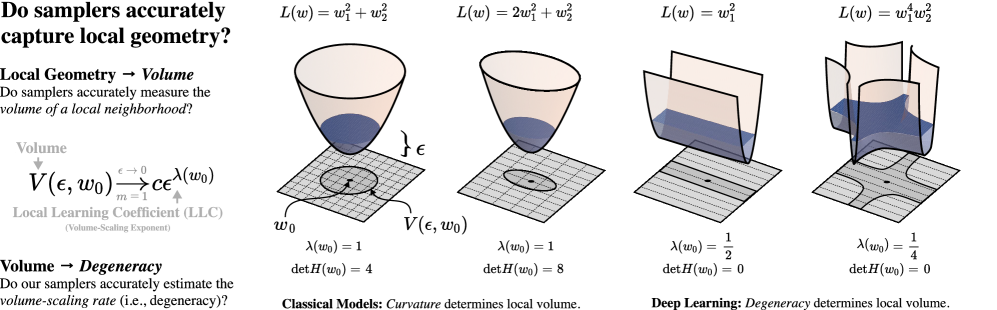
Volume scaling in the loss landscape.

An important geometric quantity of $L(w)$ from the perspective of $\pi(w)$ is the volume of sublevel sets

V(\epsilon,w_{0})=\operatorname{vol}\{w\in W\mid L(w)\leq L(w_{0})+\epsilon\}

(3.1)

where $\epsilon>0$ , $w_{0}$ is a minimum of $L(w)$ and $W\subseteq\mathbb{R}^{d}$ is a neighbourhood of $w_{0}$ . The volume $V(\epsilon,w_{0})$ quantifies the number of parameters near $w_{0}$ which achieve close to minimum loss within $W$ , and so is closely related to how the posterior distribution $\pi(w)$ concentrates.¹¹1This is notwithstanding the difference between $L_{n}(w)$ and $L(w)$ , which requires a careful technical treatment that goes beyond the scope of this paper; see Watanabe (2009, Chapter 5).

We can consider the rate of volume scaling by taking $\epsilon\to 0$ . When $w_{0}$ is a non-degenerate critical point, volume scaling is determined by the spectrum of the Hessian $H(w_{0})$ at $w_{0}$ and we have

V(\epsilon,w_{0})\approx|\det H(w_{0})|^{-1/2}\epsilon^{d/2}\qquad\text{as}~\epsilon\to 0

(3.2)

where $d$ is the dimension of parameter space. However, when $w_{0}$ is a degenerate critical point we have $\det H(w_{0})=0$ and this formula is no longer true; the second-order Taylor expansion of $L(w)$ at $w_{0}$ used to derive (3.2) no longer provides sufficient geometric information understand how volume is changing as $\epsilon\to 0$ . In general we have

V(\epsilon,w_{0})\approx c\epsilon^{\lambda(w_{0})}(-\log\epsilon)^{m(w_{0})-1}\qquad\text{as}~\epsilon\to 0

(3.3)

for some $c>0$ , where $\lambda(w_{0})\in\mathbb{Q}$ is the local learning coefficient (LLC) and $m(w_{0})\in\mathbb{N}$ is its multiplicity within $W$ (see Lau et al., 2024, Section 3, Appendix A). When $w_{0}$ is non-degenerate and the only critical point in $W$ then $\lambda(w_{0})=d/2$ , $c=|\det H(w_{0})|^{-1/2}$ and $m(w_{0})=1$ , and (3.2) is obtained from (3.3).

Measuring volume scaling via sampling.

A SGMCMC algorithm which is producing good posterior samples from a neighbourhood of $w_{0}$ should reflect the correct volume scaling rate $\lambda(w_{0})$ in (3.3). In other words, it should produce good estimates of the LLC. The LLC can be estimated by sampling from the posterior distribution (2.1) without direct access to $L(w)$ .

Definition 3.1 (Lau et al., 2024, Definition 1).

Let $w_{0}$ be a local minimum of $L(w)$ and let $W$ be an open, connected neighbourhood of $w_{0}$ such that the closure $\overline{W}$ is compact, $L(w_{0})=\inf_{w\in\overline{W}}L(w)$ , and $\lambda(w_{0})\leq\lambda(w)$ for any $w\in\overline{W}$ which satisfies $L(w)=L(w_{0})$ . The local learning coefficient estimator $\hat{\lambda}(w_{0})$ at $w_{0}$ is

\hat{\lambda}(w_{0})=n\beta(\mathbf{E}^{\beta}_{w}[L_{n}(w)]-L_{n}(w_{0}))

(3.4)

where $\mathbf{E}^{\beta}_{w}$ is an expectation over the tempered posterior (2.1) with prior $\varphi(w)$ and support $\overline{W}$ .

The following theorem and Theorem 3.4 in the next section rely on a number of technical conditions, which we give in Definition E.1 in Appendix E:

Theorem 3.2 (Watanabe, 2013, Theorem 4).

Let $w_{0}$ be a local minimum of $L(w)$ and consider the local learning coefficient estimator $\hat{\lambda}(w_{0})$ . Let the inverse temperature in (2.1) be $\beta=\beta_{0}/\log n$ for some $\beta_{0}>0$ . Then, assuming the fundamental conditions of SLT (Definition E.1), we have

$\hat{\lambda}(w_{0})$ is an asymptotically unbiased estimator of $\lambda(w_{0})$ as $n\to\infty$ .

If $q(x)=p(x|w_{0})$ for some $w_{0}\in W$ then

\operatorname{Var}(\hat{\lambda}(w_{0}))\leq\frac{\lambda(w_{0})\beta_{0}}{2\log(n)}+O\left(\frac{\lambda(w_{0})^{1/2}\beta_{0}^{3/2}}{\log(n)^{3/2}}\right)+O\left(\frac{\beta_{0}^{2}}{\log(n)^{2}}\right)\qquad\text{as }n\to\infty.

Enforcing locality in practice.

In Lau et al. (2024), locality of $\hat{\lambda}(w_{0})$ is enforced by using a Gaussian prior $\varphi(w)=\left(\gamma/\pi\right)^{d/2}\exp(-\gamma\|w-w_{0}\|^{2})$ centred at $w_{0}$ , where $\gamma>0$ is a hyperparameter of the estimator. We use the same prior in our experiments, acknowledging that this deviates from the theory above because it is not compactly supported. The way we use the prior in each sampling algorithm is made explicit in the pseudocode in Section D.3.

3.2 Deep linear network benchmark

As noted in Section 2.1, we lack theoretical convergence guarantees for SGMCMC algorithms in models such as neural networks. In the absence of these theoretical guarantees, we can instead empirically verify that samplers respect certain geometric invariants of the log-likelihood function. The local learning coefficient (LLC) from Section 3.1 is a natural choice.

We do not have ground-truth values for the LLC for most systems; the only known method for computing it exactly (i.e., other than via the estimator in Definition 3.1) involves computing a resolution of singularities (Hironaka, 1964), making the problem intractable in general. However, LLC values have recently been computed for deep linear networks (DLNs; Aoyagi, 2024). DLNs provide a scalable setting where the ground-truth LLC values are known.

Definition 3.3.

A deep linear network (DLN) with $M$ layers of sizes $H_{0},\ldots,H_{M}$ is a family of functions $f(-;\boldsymbol{w}):\mathbb{R}^{N}\to\mathbb{R}^{N^{\prime}}$ parametrised by vectors of matrices $\boldsymbol{w}=(W_{1},\ldots,W_{M})$ where $W_{l}$ is a $H_{l}\times H_{l-1}$ matrix. We define $f(x;\boldsymbol{w})=Wx$ where $W=W_{M}W_{M-1}\cdots W_{1}$ and $N=H_{0}$ , $N^{\prime}=H_{M}$ .

The learning task takes the form of a regression task using the parametrised family of DLN functions defined in Definition 3.3, with the aim being to learn the function specified by an identified parameter $\boldsymbol{w}_{0}$ . We fix integers $M$ and $H_{0},\ldots,H_{M}$ for the number of layers and layer sizes of a DLN architecture, and let $N=H_{0}$ and $N^{\prime}=H_{M}$ . We fix a prior $\varphi(\boldsymbol{w})$ on the set of all matrices parametrizing the DLN. Consider an input distribution $q(x)$ on $\mathbb{R}^{N}$ and a fixed input dataset $X_{1},\ldots,X_{n}$ drawn independently from $q(x)$ . For a parameter $\boldsymbol{w}$ , we consider noisy observations of the function’s behaviour $f(X_{i};\boldsymbol{w})+N_{i}$ , where $N_{i}\sim\mathcal{N}(0,\sigma^{2}I_{N^{\prime}})$ are independent. The likelihood of observing $(x,y)$ generated using $q(x)$ and the parameter $\boldsymbol{w}$ is

p(x,y|\boldsymbol{w})=\frac{1}{(2\pi\sigma^{2})^{N^{\prime}/2}}\exp\left(-\frac{1}{2\sigma^{2}}\|y-f(x;\boldsymbol{w})\|^{2}\right)q(x).

(3.5)

We fix $\boldsymbol{w}_{0}=(W_{1}^{(0)},\ldots,W_{M}^{(0)})$ and consider the task of learning the distribution $q(x,y)=p(x,y|\boldsymbol{w}_{0})$ . Note that while we identify a single true parameter $\boldsymbol{w}_{0}$ , when $M>1$ there are infinitely many $\boldsymbol{w}_{0}^{\prime}\neq\boldsymbol{w}_{0}$ such that $f(x;\boldsymbol{w}_{0}^{\prime})=f(x;\boldsymbol{w}_{0})$ . The dataset is $D_{n}=\{(X_{1},Y_{1}),\ldots,(X_{n},Y_{n})\}$ where $Y_{i}=f(X_{i};\boldsymbol{w}_{0})+N_{i}$ . We define

L(\boldsymbol{w})=\int_{\mathbb{R}^{N}}\|f(x;\boldsymbol{w})-f(x;\boldsymbol{w}_{0})\|^{2}q(x)dx

(3.6)

which is, up to an additive constant, the expected negative log-likelihood $-\mathbf{E}\left[p(X,Y|\boldsymbol{w})\right]$ where $(X,Y)\sim q(x,y)$ . This can be estimated using the dataset $D_{n}$ as

L_{n}(\boldsymbol{w})=\frac{1}{n}\sum_{i=1}^{n}\|Y_{i}-f(X_{i};\boldsymbol{w})\|^{2}.

(3.7)

While a DLN with $M\geq 2$ layers expresses exactly the same functions as a DLN with $M=1$ layer, the geometry of its parameter space is significantly more complex. When $M\geq 2$ the loss landscape has degenerate critical points, whereas when $M=1$ all critical points are non-degenerate. Aoyagi (2024) recently computed the LLC for DLNs, and we give this result in Theorem 3.4 below. We also refer readers to Lehalleur and Rimányi (2024).

Theorem 3.4 (Aoyagi, 2024, Theorem 1).

Consider a $M$ -layer DLN with layer sizes $H_{0},\ldots,H_{M}$ learning the regression task described above. Let $r=\operatorname{rank}(W_{M}^{(0)}W_{M-1}^{(0)}\cdots,W_{1}^{(0)})$ and $\Delta_{i}=H_{i}-r$ . There exists a set of indices $\Sigma\subseteq\{0,1,\ldots,M\}$ which satisfies:

$\max\left\{\Delta_{\sigma}\mid\sigma\in\Sigma\right\}<\min\left\{\Delta_{\overline{\sigma}}\mid\overline{\sigma}\in\Sigma^{c}\right\}$
$\sum_{\sigma\in\Sigma}\Delta_{\sigma}\geq\ell\cdot\max\left\{\Delta_{\sigma}\mid\sigma\in\Sigma\right\}$
$\sum_{\sigma\in\Sigma}\Delta_{\sigma}<\ell\cdot\max\left\{\Delta_{\overline{\sigma}}\mid\overline{\sigma}\in\Sigma^{c}\right\}$

where $\ell=|\Sigma|-1$ and $\Sigma^{c}=\{0,1,\ldots,M\}\setminus\Sigma$ . Assuming the fundamental conditions of SLT (Definition E.1), the LLC $\lambda(\boldsymbol{w}_{0})$ at the identified true parameter $\boldsymbol{w}_{0}$ is

\lambda(\boldsymbol{w}_{0})=\tfrac{1}{2}(r(H_{0}+H_{M})-r^{2})+\tfrac{1}{4\ell}a(\ell-a)-\tfrac{1}{4\ell}(\ell-1)\left(\sum_{\sigma\in\Sigma}\Delta_{\sigma}\right)^{2}+\tfrac{1}{2}\sum_{(\sigma,\sigma^{\prime})\in\Sigma^{(2)}}\Delta_{\sigma}\Delta_{\sigma^{\prime}}

where $a=\sum_{\sigma\in\Sigma}\Delta_{\sigma}-\ell\left(\left\lceil\tfrac{1}{\ell}\sum_{\sigma\in\Sigma}\Delta_{\sigma}\right\rceil-1\right)$ , $x\mapsto\lceil x\rceil$ is the ceiling function, and $\Sigma^{(2)}=\{(\sigma,\sigma^{\prime})\in\Sigma\times\Sigma\mid\sigma<\sigma^{\prime}\}$ is the set of all 2-combinations of $\Sigma$ .

3.3 Deep linear network experiments

We generate learning problems in the same way as Lau et al. (2024). We consider four classes of DLN architecture 100K, 1M, 10M and 100M, whose names correspond approximately to the number of parameters of DLNs within that class. Each class is defined by integers $M_{\text{min}}$ , $M_{\text{max}}$ and $H_{\text{min}}$ , $H_{\text{max}}$ , specifying the minimum and maximum number of layers, and minimum and maximum layer size respectively (see Table 1 in Appendix D). A learning problem is generated by randomly generating an architecture within a given class, and then randomly generating a low rank true parameter $\boldsymbol{w}_{0}$ (a detailed procedure is given in Section D.1). The input distribution is uniform on $[-10,10]^{N}$ where $N$ is the number of neurons in the input layer.

We estimate the LLC by running a given SGMCMC algorithm for $T$ steps starting at $\boldsymbol{w}_{0}$ . We provide pseudocode for our implementation Section D.3; notably the adaptive elements of AdamSGLD and RMSPropSGLD are based only on the statistics of the loss gradient and not the prior.

This results in a sequence $\boldsymbol{w}_{0},\boldsymbol{w}_{1},\ldots,\boldsymbol{w}_{T}$ of parameters. For all SGMCMC algorithms we use mini-batch estimates $L_{m,t}(\boldsymbol{w}_{t})$ of $L_{n}(\boldsymbol{w}_{t})$ , where $L_{m,t}(\boldsymbol{w}_{t})=\tfrac{1}{m}\sum\nolimits_{j=1}^{m}\|f(X_{u_{j,t}};\boldsymbol{w}_{t})-Y_{u_{j,t}}\|^{2}$ and $U_{t}=(u_{1,t},\ldots,u_{m,t})$ defines $t$ -th batch of the dataset $D_{n}$ . Rather than using $L_{n}(\boldsymbol{w}_{t})$ to estimate the LLC, instead assume that $\overline{L}\approx\mathbf{E}^{\beta}_{\boldsymbol{w}}L_{n}(\boldsymbol{w})$ where $\overline{L}=\tfrac{1}{T-B}\sum\nolimits_{t=B}^{T}L_{m,t}(\boldsymbol{w}_{t})$ for some number of ‘burn-in’ steps $B$ . Inspired by Definition 3.1, we then estimate the LLC at $\boldsymbol{w}_{0}$ as

\overline{\lambda}(\boldsymbol{w}_{0})\coloneqq n\beta(\overline{L}-L_{m,0}(\boldsymbol{w}_{0})).

(3.8)

To improve this estimate, one could run $C>1$ independent sampling chains to obtain estimates however in this case we take $C=1$ , preferring instead to run more experiments with different architectures. We give the hyperparameters used in LLC estimation in Table 2 in Appendix D.

4 Results

To assess how well they capture the local posterior geometry, we apply the benchmark described in Section 3.2 to the following samplers: SGLD (Welling and Teh, 2011), SGLD with RMSProp preconditioning (RMSPropSGLD; Li et al. 2016), an “Adam-like” adaptive SGLD (AdamSGLD; Kim et al. 2020), SGHMC (Chen et al., 2014) and SGNHT (Ding et al., 2014). We give pseudocode for our implementation these samplers in Section D.3. We are interested not only in the absolute performance of a given sampler, but also in how sensitive its estimates are to the chosen step size $\epsilon$ of the sampler. To assess the performance of a sampler at a given step size, we primarily consider the relative error $(\hat{\lambda}-\lambda)/\lambda$ of an LLC estimate $\hat{\lambda}$ with true value $\lambda$ .

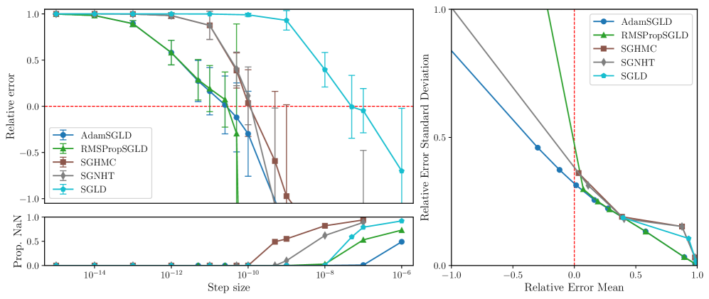
RMSPropSGLD and AdamSGLD are less sensitive to step-size.

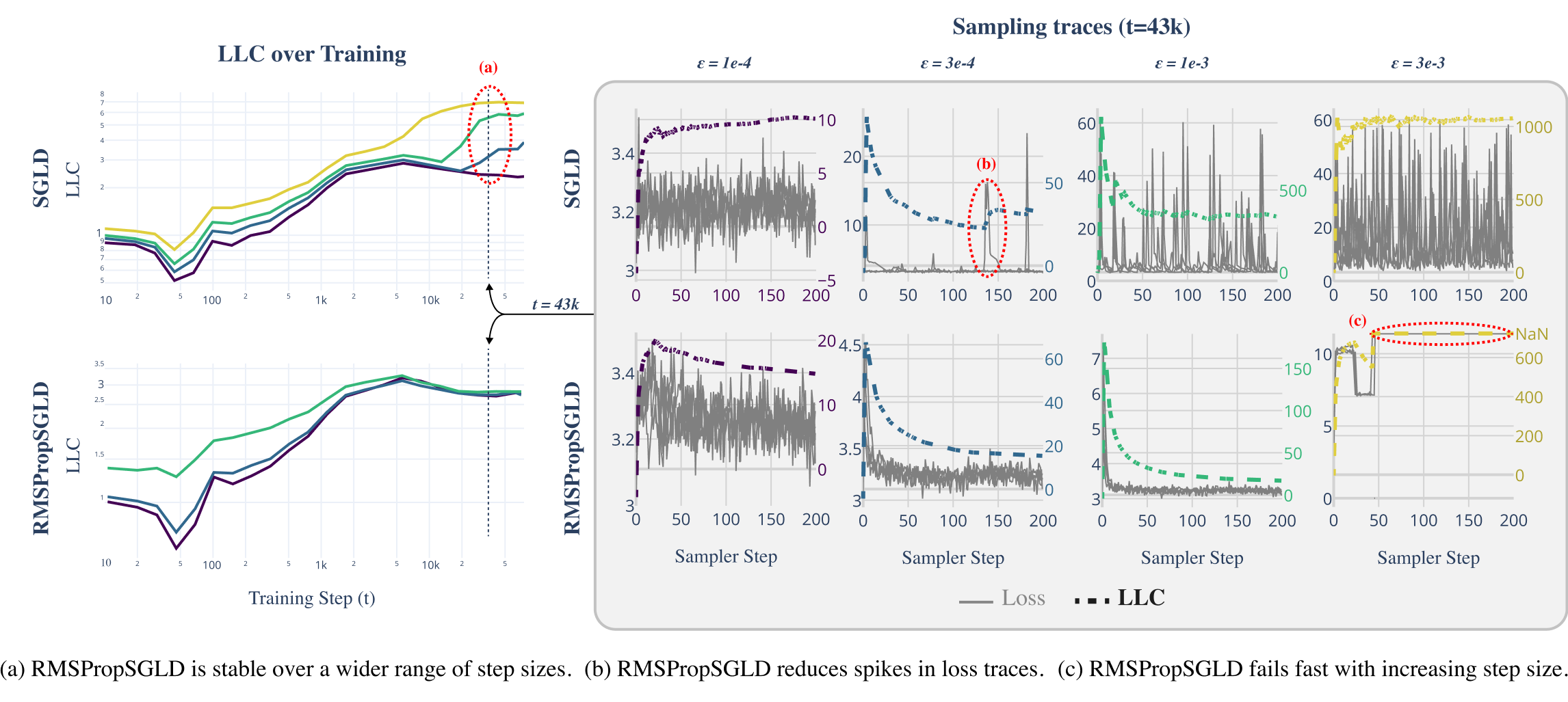
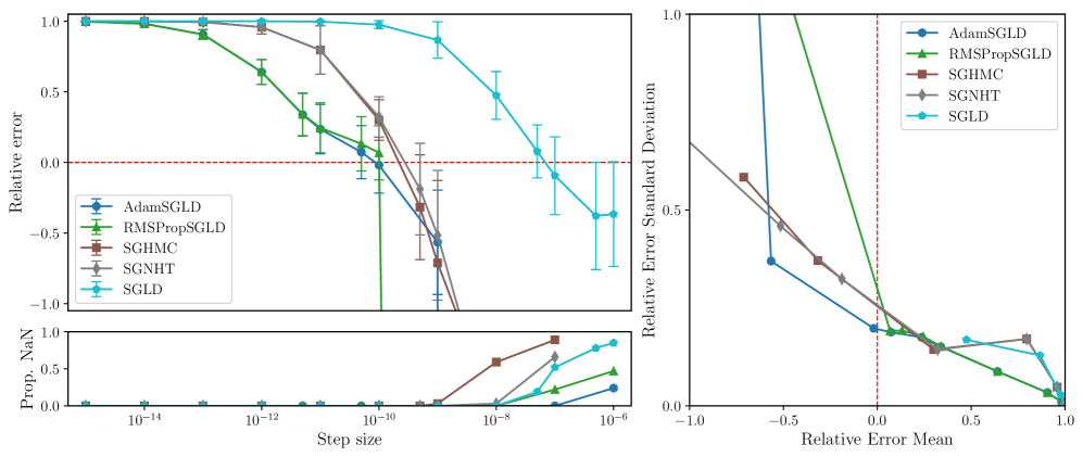
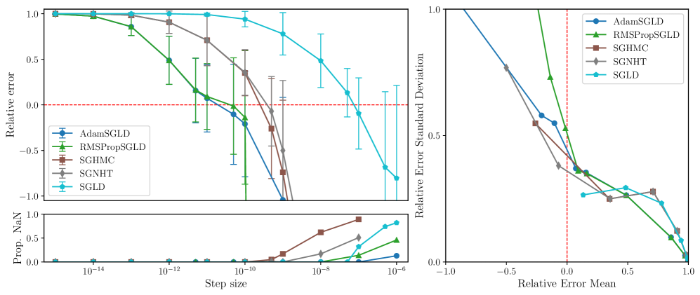
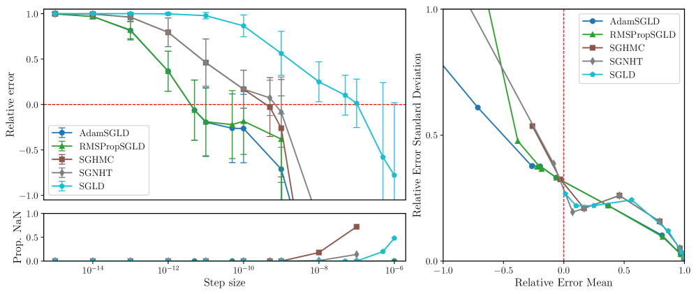
Figures 3, 5, 6 and 7 display the mean relative error (averaged over different networks generated from the model class) versus the step size of each sampler. While all samplers seem to be able to achieve empirically unbiased LLC estimates (relative error = 0) for some step size, RMSPropSGLD and AdamSGLD have a wider range of step size values which produce accurate results. For SGLD, at the step size values where the relative error is close to zero, a significant fraction of the LLC estimates are also diverging. In experiments on language models (Figure 4), RMSPropSGLD is also stable across a wider range of step sizes . This results in more consistent LLC estimates compared to SGLD.

RMSPropSGLD and AdamSGLD achieve a superior mean-variance tradeoff.

In Figures 3, 5, 6 and 7 we plot the mean of the relative error versus the standard deviation of the relative error for each sampler at different step sizes. We see that RMSPropSGLD and AdamSGLD obtain a superior combination of good mean performance and lower variance compared to the other samplers.

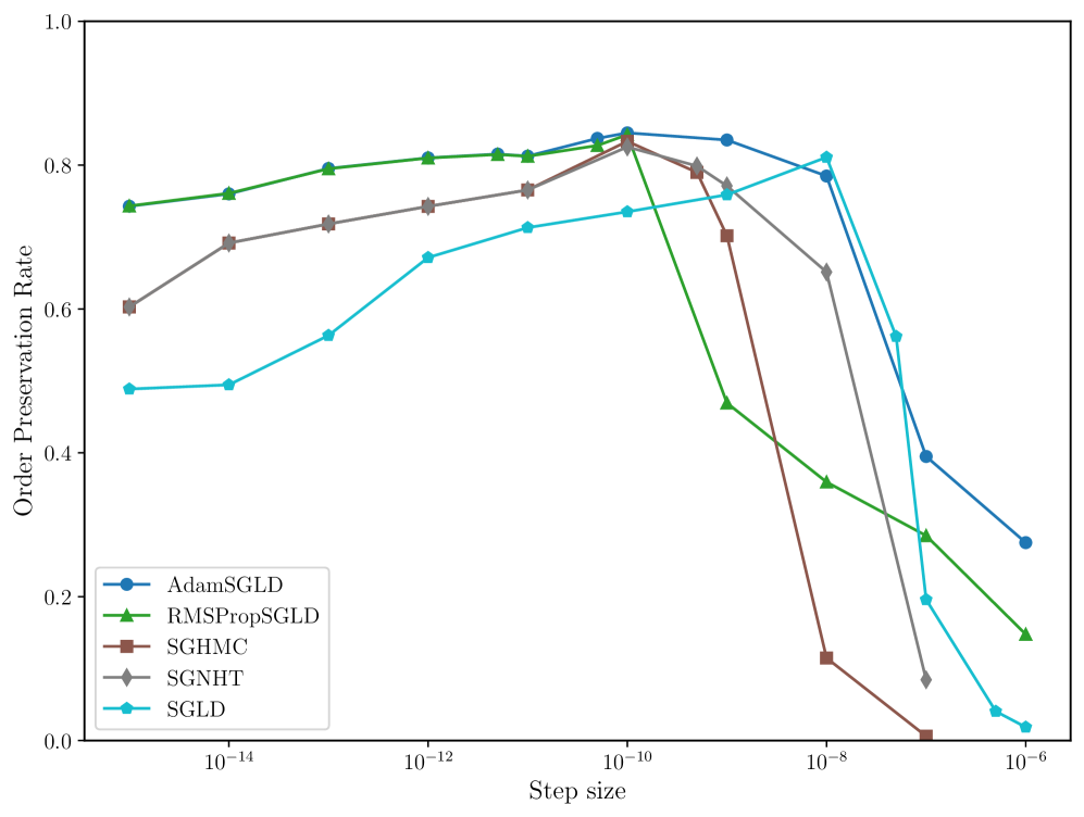
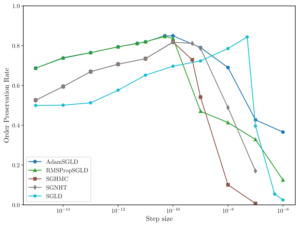
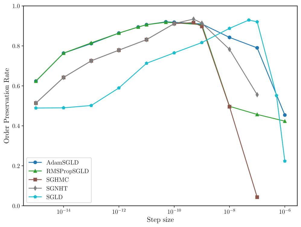
RMSPropSGLD and AdamSGLD are better at preserving order.

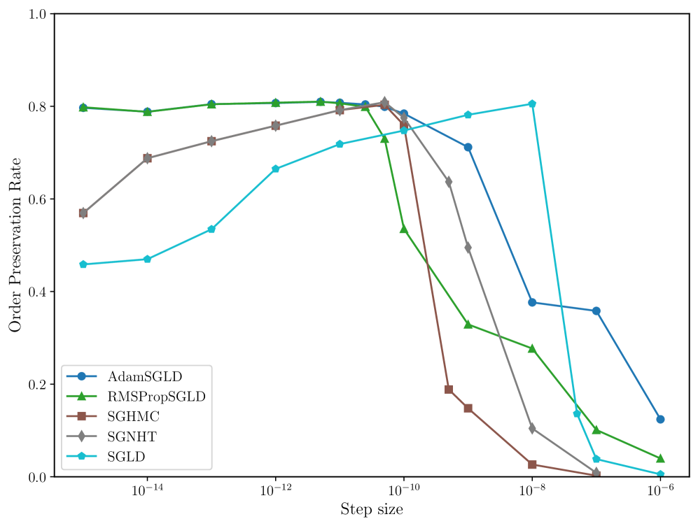
In many applications of LLC estimation, observing relative changes (e.g. over training) in the LLC is more important than determining absolute values (Chen et al., 2023; Hoogland et al., 2025; Wang et al., 2024). In these cases, the order of a sampler’s estimates should reflect the order of the true LLCs. We compute the order preservation rate of each sampler, which we define as the proportion of all pairs of estimates for which the order of the true LLCs matches the estimates. We plot this quantity versus the step size in Figure 8 in Appendix C. Again, RMSPropSGLD and AdamSGLD achieve superior performance to the other samplers with a higher order preservation rate across a wider range of step sizes.

RMSPropSGLD step size is easier to tune.

Above a certain step size RMSPropSGLD experiences rapid performance degradation, with LLC estimates which are orders of magnitude larger than the maximum theoretical value of $d/2$ and large spikes in the loss trace of the sampler. In contrast, AdamSGLD experiences a more gradual performance degradation and its loss traces do not obviously suggest the step size is set to high. We see this catastrophic drop-off in performance as an advantage of RMSPropSGLD, as it provides a clear signal that hyperparameters are incorrectly tuned in the absence of ground-truth LLC values. This clear signal is not present for AdamSGLD.

5 Discussion

In this paper we introduced a scalable benchmark for evaluating the local sampling performance of SGMCMC algorithms. This benchmark is based on how well samplers estimate the local learning coefficient (LLC) for deep linear networks (DLNs). Since the LLC is the local volume-scaling rate for the log-likelihood function, this directly assesses how well samplers explore the local posterior.

Towards future empirical benchmarks.

The stochastic optimization literature has accumulated numerous benchmarks for assessing (optimization) performance on non-convex landscapes (e.g., Rastrigin, Ackley, and Griewank functions; Plevris and Solorzano 2022). However, these benchmarks focus primarily on multimodality and often ignore degeneracy. Our current work takes DLNs as an initial step towards developing a more representative, degeneracy-aware benchmark. A key limitation is that DLNs represent only one class of degenerate models and may not capture all forms of degeneracy encountered in general (see Lehalleur and Rimányi, 2024). Developing a wider set of degeneracy-aware benchmarks therefore remains an important direction for future research.

Towards future theoretical guarantees.

In Section 2.1, we establish that global convergence guarantees for sampling algorithms like SGLD rely on assumptions which provably do not hold for certain model classes (e.g. deep linear networks) with degenerate loss landscapes, and are unlikely to be compatible with degeneracy in general. Shifting from global to local convergence guarantees, which properly account for degeneracy, provides one promising way forward.

This shift may have broader implications beyond sampling. Many current convergence guarantees for stochastic optimizers make similar assumptions that may fail for degenerate landscapes (e.g., global Lipschitz or Polyak-Łojasiewicz conditions; Rebjock and Boumal 2024). Generally, the role of degeneracy in shaping the dynamics of sampling and optimization methods is not well understood.

Open problem: A theoretical explanation for the empirical success of local SGMCMC.

In this paper, we observed empirically that SGMCMC algorithms can successfully estimate the LLC despite the lack of theoretical convergence guarantees. The strong assumptions employed by the convergence results discussed in Section 2.1 arise, in some sense, because the goal is to prove global convergence to a posterior with support $\mathbb{R}^{d}$ . It possible is that convergence results similar to those in Section 2.1 may be proved for compact parameter spaces, however this does not explain the success of local sampling we observe because our experiments are not in a compactly supported setting. This also places our empirical results outside of the setting of SLT (in particular Theorem 3.2 and Theorem 3.4). We see understanding precisely what determines the “effective support” of SGMCMC sampling chains in practice as a central issue in explaining why these samplers work in practice.

Appendix

This appendix contains supplementary details, proofs, and experimental results supporting the main text. Specifically, we include:

Appendix A provides examples of global and local degeneracies that are characteristic of modern deep neural network architectures.
Appendix B provides a proof of Lemma 2.1, which shows that the negative log-likelihood of deep linear networks is a polynomial of degree $2M$ .
Appendix C presents additional experimental results, focusing on the relative error, variance, and order preservation rates of various samplers across different deep linear network architectures.
Appendix D describes additional methodological details, including procedures for randomly generating deep linear network tasks, explicit hyperparameter settings for LLC estimation, and pseudocode for the implemented SGMCMC algorithms.
Appendix E summarizes the fundamental technical conditions required by singular learning theory (SLT), outlining the mathematical assumptions underlying our theoretical discussions.

Appendix A Examples of Degeneracy

Degenerate critical points in the loss landscape of neural networks can arise from symmetries in the parametrisation: continuous (or discrete) families of parameter settings that induce identical model outputs or leave the training loss unchanged. We distinguish global (or “generic”) symmetries, which hold throughout parameter space, from local and data-dependent degeneracies that arise only in particular regions in parameter space or only for particular data distributions. In this section we provide several examples (these are far from exhaustive).

A.1 Global degeneracies

Matrix–sandwich symmetry in deep linear networks.

For a DLN with composite weight $W=W_{M}\cdots W_{1}$ one can insert any invertible matrix $O$ between any neighbouring layers, e.g., $W=(W_{M}O)(O^{-1}W_{M-1})W_{M-2}\!\dotsm W_{1},$ without changing the implemented function. This produces a $\,\mathrm{GL}(H)$ –orbit of equivalent parameters.

ReLU scaling symmetries.

Because $\operatorname{ReLU}(ax)=a\,\operatorname{ReLU}(x)$ for all $a>0$ , scaling pre–activation weights by $a$ and post–activation weights by $a^{-1}$ leaves the network invariant. Such positively scale–invariant (PSI) directions invalidate naïve flatness measures [Yi et al., 2019, Tsuzuku et al., 2020].

Permutation and sign symmetries.

Exchanging hidden units (or simultaneously flipping signs of incoming and outgoing weights) are examples of discrete changes that leave network outputs unchanged [Carroll, 2021].

Batch- and layer-normalization scaling symmetries.

BN and LN outputs do not change when their inputs pass through the same affine map [Laarhoven, 2017].

A.2 Local and data-dependent degeneracies

Low-rank DLNs.

When the end-to-end matrix $W$ is rank-deficient, any transformation restricted to the null space can be absorbed by the factors $W_{\ell}$ .

Elimination singularities.

If incoming weights to a given layer are zero, the associated outgoing weights are free to take any value. The reverse also holds: if outgoing weights are zero, this frees incoming weights to take any value. Residual or skip connections can help to bypass these degeneracies [Orhan and Pitkow, 2018].

Dead (inactive) ReLUs.

If a bias is large enough that a ReLU never activates or if the data distribution is such that the pretraining activations never exceed the bias, then the outgoing weights become free parameters; they can be set to arbitrary values without affecting loss because they are always multiplied by a zero activation. Incoming weights also become free parameters (up until the point that they change the preactivation distribution enough to activate the ReLU).

Always-active ReLUs.

Conversely, ReLUs that are always on behave linearly. In this regime, the incoming and outgoing weight matrices act as a DLN with the associated matrix-sandwich and low-rank degeneracies discussed above.

Overlap singularities.

If two neurons share the same incoming weights, then the outgoing weights become non-identifiable: in this regime, only the sum matters to the model’s functional behaviour [Orhan and Pitkow, 2018].

Appendix B Proof of Lemma 2.1

In this section we prove Lemma 2.1, which shows that the global convergence results for SGLD discussed in Section 2.1 do not apply to the regression problem for deep linear networks described in Section 3.2.

Consider an $M$ -layer deep linear network with layer sizes $H_{0},\ldots,H_{M}$ . Recall from Definition 3.3 that this is a family of functions $f(-;\boldsymbol{w}):\mathbb{R}^{N}\to\mathbb{R}^{N^{\prime}}$ parametrised by matrices $\boldsymbol{w}=(W_{1},\ldots,W_{M})$ where $W_{l}$ is $H_{l}\times H_{l-1}$ and $N=H_{0}$ and $N^{\prime}=H_{M}$ . By definition we have

f(x;\boldsymbol{w})=W_{M}W_{M-1}\cdots W_{1}x.

We consider the regression task described in Section 3. Let $q(x)$ be an absolutely continuous input distribution on $\mathbb{R}^{N}$ and $X_{1},\ldots,X_{n}$ be an input dataset drawn from independently from $q(x)$ . For an identified parameter $\boldsymbol{w}_{0}=(W_{1}^{(0)},\ldots,W_{M}^{(0)})$ we consider the task of learning the function $f(x;\boldsymbol{w}_{0})$ . That is, we consider the statistical model

p(x,y|\boldsymbol{w})=\frac{1}{(2\pi\sigma^{2})^{N^{\prime}/2}}\exp\left(-\frac{1}{2\sigma^{2}}\|y-f(x;\boldsymbol{w})\|^{2}\right)q(x)

from (3.5), where the true distribution is $q(x,y)=p(x,y|\boldsymbol{w}_{0})$ . As in (3.6) and (3.7) we consider

L(\boldsymbol{w})=\int_{\mathbb{R}^{N}}\|f(x;\boldsymbol{w})-f(x;\boldsymbol{w}_{0})\|^{2}q(x)dx

and

L_{n}(\boldsymbol{w})=\frac{1}{n}\sum_{i=1}^{n}\|f(X_{i};w)-f(X_{i};w_{0})\|^{2}.

which are, up to additive constants (irrelevant when computing gradients), the expected and empirical negative log-likelihood respectively. When sampling from the tempered posterior distribution (2.1) using a Langevin diffusion based sampler like SGLD, $\nabla L_{n}(w)$ is used to compute sampler steps along with the prior and noise terms (see Section 2.1).

For convenience in the following proof, and in-line with the experimental method in Section 3.3, we consider a prior which is an isotropic Gaussian distribution on $\boldsymbol{w}$

\varphi(\boldsymbol{w})=\left(\frac{\gamma}{2\pi}\right)^{d/2}\exp\left(-\frac{\gamma}{2}\|\boldsymbol{w}-\boldsymbol{w}_{\mu}\|^{2}\right)

(B.1)

where $\gamma>0$ and $\boldsymbol{w}_{\mu}$ is any fixed parameter. By $\|\boldsymbol{w}-\boldsymbol{w}_{\mu}\|^{2}$ we mean to take the sum of the square of all matrix entries, treating the parameter $\boldsymbol{w}$ in this expression as a vector with $d=\sum_{l=1}^{M}H_{l}H_{l-1}$ entries.

Lemma B.1 (restating Lemma 2.1).

Consider the above situation of an $M$ -layer deep linear network learning the described regression task. If $q(x)$ is absolutely continuous then with probability one $L_{n}(\boldsymbol{w})$ is a degree $2M$ polynomial in the matrix entries $\boldsymbol{w}=(W_{1},\ldots,W_{M})$ .

Proof.

We treat each parameter of the model as a different polynomial variable; that is, for each $l=1,\ldots M$ we have $W_{l}=(w^{l}_{i,j,l})$ where $w_{i,j,l}$ are distinct polynomial variables. As before let $W=W_{M}W_{M-1}\cdots W_{1}$ . For a matrix $U$ with polynomial entries we denote by $\deg(U)$ the maximum degree of its entries. Hence we have that $\deg(W)=M$ since each entry of $W$ is a sum of monomials of the form $\prod_{l=1}^{M}w_{i_{l},j_{l},l}$ . Denote the entries of $W$ by $P_{ij}(\boldsymbol{w})$ , which is a polynomial of degree $M$ in the variables $w_{i,j,l}$ . The entries of $W^{(0)}$ are constants, and we denote them by $a_{ij}$ .

We now consider the degree of the likelihood function $L_{n}(\boldsymbol{w})$ as a polynomial in the variables $w_{i,j,l}$ . Let $N=H_{0}$ denote the input dimension of the deep linear network and $N^{\prime}=H_{M}$ the output dimension. First note that square of the $i$ -th coordinate of $WX_{k}-W^{(0)}X_{k}$ is

	$\displaystyle(WX_{k}-W^{0}X_{k})_{i}^{2}$	$\displaystyle=\left(\sum_{j=1}^{N}P_{ij}(\boldsymbol{w})X_{k}^{(j)}-a_{ij}X_{k}^{(j)}\right)^{2}$
		$\displaystyle=\sum_{j=1}^{N}\sum_{j^{\prime}=1}^{N}X_{k}^{(j)}X_{k}^{(j^{\prime})}\left(P_{ij}(\boldsymbol{w})P_{ij^{\prime}}(\boldsymbol{w})-a_{ij}P_{ij^{\prime}}(\boldsymbol{w})-a_{ij^{\prime}}P_{ij}(\boldsymbol{w})+a_{ij}a_{ij^{\prime}}\right)$

where $X_{k}^{(j)}$ is the $j$ -th coordinate of $X_{k}$ . Hence we have

	$\displaystyle L_{n}(\boldsymbol{w})$	$\displaystyle=\frac{1}{n}\sum_{k=1}^{n}\sum_{i=1}^{N^{\prime}}(WX_{k}-W^{0}X_{k})_{i}^{2}$
		$\displaystyle=\frac{1}{n}\sum_{k=1}^{n}\sum_{i=1}^{N^{\prime}}\sum_{j=1}^{N}\sum_{j^{\prime}=1}^{N}X_{k}^{(j)}X_{k}^{(j^{\prime})}P_{ij}(\boldsymbol{w})P_{ij^{\prime}}(\boldsymbol{w})+\left(\text{terms of at most degree }M\right)$
		$\displaystyle=\frac{1}{n}\sum_{i=1}^{N^{\prime}}\sum_{j=1}^{N}\sum_{j^{\prime}=1}^{N}\left(\sum_{k=1}^{n}X_{k}^{(j)}X_{k}^{(j^{\prime})}\right)P_{ij}(\boldsymbol{w})P_{ij^{\prime}}(\boldsymbol{w})+\left(\text{terms of at most degree }M\right)$

The polynomial $P_{ij}(\boldsymbol{w})P_{ij^{\prime}}(\boldsymbol{w})$ has degree $2M$ . The only way $L_{n}(\boldsymbol{w})$ can have degree smaller than $2M$ is if the random coefficients $\sum_{k=1}^{n}X_{k}^{(j)}X_{k}^{(j^{\prime})}$ result in cancellation between the terms of different $P_{ij}(\boldsymbol{w})P_{ij^{\prime}}(\boldsymbol{w})$ . We now show that this does not happen with probability one. Consider a function $f:\mathbb{R}^{nN}\to\mathbb{R}$ given by

f(\boldsymbol{x})=\sum_{(b,b^{\prime})\in\Lambda}c_{bb^{\prime}}x_{b}x_{b}^{\prime}

where $\Lambda$ is any non-empty subset of $\{1,\ldots,nN\}^{2}$ and $c_{bb^{\prime}}\in\mathbb{R}\setminus\{0\}$ . The set $f^{-1}(0)\subseteq\mathbb{R}^{nN}$ has Lebesgue measure zero, and hence has measure zero with respect to the joint distribution of the dataset $D_{n}$ considered as a distribution on $\mathbb{R}^{nN}$ , since $q(x)$ is assumed to be absolutely continuous. It follows that cancellation of the degree $2M$ monomials in the above expression for $L_{n}(\boldsymbol{w})$ cannot occur with probability greater than zero, and thus $\deg(L_{n}(\boldsymbol{w}))=2M$ with probability one.

Recall from Section 2.1 that proofs about the global convergence of SGLD assume that there exists a function $V:\mathbb{R}^{d}\to[1,\infty)$ with bounded second derivatives which satisfies

\|\nabla V(\boldsymbol{w})\|^{2}+\|\nabla\log\pi(\boldsymbol{w})\|^{2}\leq CV(\boldsymbol{w})\qquad\text{ for all }w\in\mathbb{R}^{d}.

See Teh et al. [2015, Assumption 4]. In the setting of deep linear networks we have $\nabla\log\pi(\boldsymbol{w})=-n\beta\nabla L_{n}(\boldsymbol{w})$ . Since the second derivatives of $V$ are bounded and $L_{n}(\boldsymbol{w})$ is a degree $2M$ polynomial, this condition can only hold when $M=1$ . This corresponds precisely to the case when all critical points of $L_{n}(w)$ are non-degenerate. Likewise, the global Lipschitz condition

\|\nabla\log\pi(w_{1})-\nabla\log\pi(w_{2})\|\leq\alpha\|w_{1}-w_{2}\|\qquad\text{ for all }w_{1},w_{2}\in\mathbb{R}^{d}.

can also only be satisfied when $M=1$ .

Remark B.2.

In detailed treatments of singular models such as Watanabe [2009] it is often more convenient to analyse the distribution

\pi(\boldsymbol{w})\propto\exp(-n\beta L(\boldsymbol{w}))\varphi(\boldsymbol{w})

(B.2)

in-place of the tempered posterior distribution (2.1). The geometry of $L(\boldsymbol{w})$ determines much of the learning behaviour of singular statistical models. In SGMCMC algorithms, a stochastic estimate $g(\boldsymbol{w},U)$ of the gradient of the log-posterior could equally be considered an estimate of $\nabla\log\pi(\boldsymbol{w})$ , where $\pi(\boldsymbol{w})$ is as in (B.2). In the case of deep linear networks, a result similar to Lemma B.1 can be shown using (B.2) in-place of the usual posterior distribution. In this case we have

L(\boldsymbol{w})=\mathbf{E}\|WX-W^{(0)}X\|^{2}

where $X\sim q(x)$ . From the proof of Lemma B.1 we have that

	$\displaystyle L(\boldsymbol{w})$	$\displaystyle=\mathbf{E}\left[\sum_{i=1}^{N^{\prime}}\sum_{j=1}^{N}\sum_{j^{\prime}=1}^{N}X_{j}X_{j^{\prime}}P_{ij}(\boldsymbol{w})P_{ij^{\prime}}(\boldsymbol{w})\right]+\left(\text{terms of at most degree }M\right)$
		$\displaystyle=\sum_{i=1}^{N^{\prime}}\sum_{j=1}^{N}\sum_{j^{\prime}=1}^{N}\mathbf{E}\left[X_{j}X_{j^{\prime}}\right]P_{ij}(\boldsymbol{w})P_{ij^{\prime}}(\boldsymbol{w})+\left(\text{terms of at most degree }M\right).$

where we now write $X_{j}$ for the $j$ -th coordinate of $X$ . If each coordinate of $X$ is independent and identically distributed (as in the experiments in Section 3.3) then $\mathbf{E}\left[X_{j}^{2}\right]>0$ and $\mathbf{E}\left[X_{j}X_{j^{\prime}}\right]\geq 0$ for $j\neq j^{\prime}$ . It follows that $L(\boldsymbol{w})$ has degree $2M$ , since all monomial terms with degree $2M$ in the above expression for $L(\boldsymbol{w})$ appear with non-negative coefficients, and at least some are non-zero.

Appendix C Additional results

In this section we give additional results from the experiments described in Section 3.3. In Figures 5, 6 and 7 we present the relative error $(\hat{\lambda}-\lambda)/\lambda$ in the estimated local learning coefficient for the deep linear network model classes 10M, 1M and 100K (the results for the 100M model class is given in Figure 3 in the main text).

In Figure 8 we present the order preservation rate of each sampling algorithm, for each deep linear network model class. This assesses how good a sampling algorithm is at preserving the ordering of local learning coefficient estimates. These results are discussed in more detail in Section 4 in the main text.

Appendix D Additional methodology details

In this sectional methodology details, supplemental to Section 3.3. In Section D.1 we describe the procedure for generating deep linear networks, mentioned in Section 3.3. In Section D.3 we give pseudocode for the samplers we benchmark: SGLD (Algorithm 1), AdamSGLD (Algorithm 2), RMSPropSGLD (Algorithm 3), SGHMC (Algorithm 4) and SGNHT (Algorithm 5). In Section D.4 we give details of the large language model experiments presented in Figure 4.

D.1 Deep linear network generation

With the notation introduced in Section 3.3, a deep linear network is generated as follows. The values of $M_{\text{min}}$ , $M_{\text{max}}$ , $H_{\text{min}}$ and $H_{\text{max}}$ for each model class are given in Table 1.

Choose a number of layers $M$ uniformly from $\{M_{\text{min}},M_{\text{min}}+1,\ldots,M_{\text{max}}\}$ .
Choose layer sizes $H_{l}$ uniformly from $\{H_{\text{min}},H_{\text{min}}+1,\ldots,H_{\text{max}}\}$ , for $l=1,\ldots,M$ .
Generate a fixed parameter $\boldsymbol{w}_{0}=(W_{1}^{(0)},\ldots,W_{M}^{(0)})$ where $W^{(0)}_{l}$ is a $H_{l}\times H_{l-1}$ matrix generated according to the Xavier-normal distribution: each entry is drawn independently from $\mathcal{N}(0,\sigma^{2})$ where $\sigma^{2}=\tfrac{2}{H_{l}+H_{l-1}}$ .
To obtain lower rank true parameters we modify $\boldsymbol{w}_{0}$ as follows. For each layer $l=1,\ldots,M$ we choose whether or not to reduce the rank of $W_{l}$ with probability $0.5$ . If we choose to do so, we choose a new rank $r$ uniformly from $\{0,\ldots,\min(H_{l},H_{l-1})\}$ and set some number of rows or columns of $W_{l}$ to zero to force it to be at most rank $r$ .

The above process results in a deep linear network $f(x;\boldsymbol{w})$ with $M$ layers and layer sizes $H_{0},\ldots,H_{M}$ , along with an identified true parameter $\boldsymbol{w}$ . We take the input distribution to be the uniform distribution on $[-10,10]^{N}$ where $N=H_{0}$ , and the output noise distribution is $\mathcal{N}(\boldsymbol{0},\sigma^{2}I_{N^{\prime}})$ where $N^{\prime}=H_{M}$ and $\sigma^{2}=1/4$ .

	100K	1M	10M	100M
Minimum number of layers $M_{\text{min}}$	2	2	2	2
Maximum number of layers $M_{\text{max}}$	10	20	20	40
Minimum layer size $H_{\text{min}}$	50	100	500	500
Maximum layer size $H_{\text{max}}$	500	1000	2000	3000

Table 1: Deep linear network architecture hyperparameters

Number of sampling steps	$5\times 10^{4}$
Number of burn-in steps $B$	$0.9T$
Dataset size $n$	$10^{6}$
Batch size $m$	$500$
Localisation parameter $\gamma$	$1$
Inverse-temperature parameter $\beta$	$1/\log(n)$
Number of learning problems	$100$

Table 2: Hyperparameters for local learning coefficient estimation in deep linear networks.

D.2 Deep linear network compute details

The DLN experiments were run on a cluster using NVIDIA H100 GPUs. A batch of 100 independent experiments took approximately 7 GPU hours for the 100M model class, 5 GPU hours for the 10M model class, 3.5 GPU hours for the 1M model class, and 0.9 GPU hours for the 100K model class. The total compute used for the DLN experiments was approximately 1000 GPU hours.

D.3 Samplers

Algorithm 1 SGLD

1:Inputs:

\boldsymbol{w}_{0}\in\mathbb{R}^{d}

(initial parameter),

D_{n}=\{\boldsymbol{z}_{1},\ldots,\boldsymbol{z}_{n}\}

(dataset),

\ell:\mathbb{R}^{N}\times\mathbb{R}^{d}\to\mathbb{R}

(loss function)

2:Outputs:

\boldsymbol{w}_{1},\ldots,\boldsymbol{w}_{T}\in\mathbb{R}^{d}

3:Hyperparameters:

\epsilon>0

(step size),

\gamma>0

(localization),

\tilde{\beta}>0

(posterior temperature),

m\in\mathbb{N}

(batch size)

t\leftarrow 0:T-1

5:Draw a batch

z_{u_{1}},\ldots,z_{u_{m}}

from

D_{n}

\boldsymbol{g}_{t}\leftarrow\frac{1}{m}\sum_{k=1}^{m}\nabla_{\boldsymbol{w}}\ell(\boldsymbol{z}_{u_{k}},\boldsymbol{w}_{t})

\triangleright

Gradient with respect to the parameter argument.

7:Draw

\boldsymbol{\eta}_{t}

from the standard normal distribution on

\mathbb{R}^{d}

\Delta\boldsymbol{w}_{t}\leftarrow\tfrac{-\epsilon}{2}\left(\gamma(\boldsymbol{w}_{t}-\boldsymbol{w}_{0})+\tilde{\beta}\boldsymbol{g}_{t}\right)+\sqrt{\epsilon}\boldsymbol{\eta}_{t}

\boldsymbol{w}_{t+1}\leftarrow\boldsymbol{w}_{t}+\Delta\boldsymbol{w}_{t}

Algorithm 2 AdamSGLD

1:Inputs:

\boldsymbol{w}_{0}\in\mathbb{R}^{d}

(initial parameter),

D_{n}=\{\boldsymbol{z}_{1},\ldots,\boldsymbol{z}_{n}\}

(dataset),

\ell:\mathbb{R}^{N}\times\mathbb{R}^{d}\to\mathbb{R}

(loss function)

2:Outputs:

\boldsymbol{w}_{1},\ldots,\boldsymbol{w}_{T}\in\mathbb{R}^{d}

3:Hyperparameters:

\epsilon>0

(base step size),

\gamma>0

(localization),

\tilde{\beta}>0

(posterior temperature),

m\in\mathbb{N}

(batch size),

a>0

(stability),

b_{1},b_{2}\in(0,1)

(EMA decay rates)

\boldsymbol{m}_{-1}\leftarrow(0,0,\ldots,0)\in\mathbb{R}^{d}

\boldsymbol{v}_{-1}\leftarrow(1,1,\ldots,1)\in\mathbb{R}^{d}

t\leftarrow 0:T-1

7:Draw a batch

z_{u_{1}},\ldots,z_{u_{m}}

from

D_{n}

\boldsymbol{g}_{t}\leftarrow\frac{1}{m}\sum_{k=1}^{m}\nabla_{\boldsymbol{w}}\ell(\boldsymbol{z}_{u_{k}},\boldsymbol{w}_{t})

\triangleright

Gradient with respect to the parameter argument.

\boldsymbol{m}_{t}\leftarrow b_{1}\boldsymbol{m}_{t-1}+(1-b_{1})\boldsymbol{g}_{t}

10:Define

\boldsymbol{v}_{t}

\boldsymbol{v}_{t}[i]\leftarrow b_{2}\boldsymbol{v}_{t-1}[i]+(1-b_{2})\boldsymbol{g}_{t}[i]^{2}

for

i=1,\ldots,d

11:

\hat{\boldsymbol{m}}_{t}\leftarrow\frac{1}{1-b_{1}^{t}}\boldsymbol{m}_{t}

12:

\hat{\boldsymbol{v}}_{t}\leftarrow\frac{1}{1-b_{2}^{t}}\boldsymbol{v}_{t}

13:Define

\boldsymbol{\epsilon}_{t}

\boldsymbol{\epsilon}_{t}[i]\leftarrow\frac{\epsilon}{\sqrt{\hat{\boldsymbol{v}}_{t}[t]}+a}

for

i=1,\ldots,d

\triangleright

Step size of each parameter.

14:Draw

\boldsymbol{\eta}_{t}

from the standard normal distribution on

\mathbb{R}^{d}

15:Define

\Delta\boldsymbol{w}_{t}

\Delta\boldsymbol{w}_{t}[i]\leftarrow\tfrac{-\boldsymbol{\epsilon}_{t}[i]}{2}\left(\gamma(\boldsymbol{w}_{t}[i]-\boldsymbol{w}_{0}[i])+\tilde{\beta}\hat{\boldsymbol{m}}_{t}[i]\right)+\sqrt{\boldsymbol{\epsilon}_{t}[i]}\boldsymbol{\eta}_{t}[i]

for

i=1,\ldots,d

16:

\boldsymbol{w}_{t+1}\leftarrow\boldsymbol{w}_{t}+\Delta\boldsymbol{w}_{t}

Algorithm 3 RMSPropSGLD

1:Inputs:

\boldsymbol{w}_{0}\in\mathbb{R}^{d}

(initial parameter),

D_{n}=\{\boldsymbol{z}_{1},\ldots,\boldsymbol{z}_{n}\}

(dataset),

\ell:\mathbb{R}^{N}\times\mathbb{R}^{d}\to\mathbb{R}

(loss function)

2:Outputs:

\boldsymbol{w}_{1},\ldots,\boldsymbol{w}_{T}\in\mathbb{R}^{d}

3:Hyperparameters:

\epsilon>0

(base step size),

\gamma>0

(localization),

\tilde{\beta}>0

(posterior temperature),

m\in\mathbb{N}

(batch size),

a>0

(stability),

b\in(0,1)

(EMA decay rate)

\boldsymbol{v}_{-1}\leftarrow(1,1,\ldots,1)\in\mathbb{R}^{d}

t\leftarrow 0:T-1

6:Draw a batch

z_{u_{1}},\ldots,z_{u_{m}}

from

D_{n}

\boldsymbol{g}_{t}\leftarrow\frac{1}{m}\sum_{k=1}^{m}\nabla_{\boldsymbol{w}}\ell(\boldsymbol{z}_{u_{k}},\boldsymbol{w}_{t})

\triangleright

Gradient with respect to the parameter argument.

8:Define

\boldsymbol{v}_{t}

\boldsymbol{v}_{t}[i]\leftarrow b\boldsymbol{v}_{t-1}[i]+(1-b)\boldsymbol{g}_{t}[i]^{2}

for

i=1,\ldots,d

\hat{\boldsymbol{v}}_{t}\leftarrow\frac{1}{1-b^{t}}\boldsymbol{v}_{t}

10:Define

\boldsymbol{\epsilon}_{t}

\boldsymbol{\epsilon}_{t}[i]\leftarrow\frac{\epsilon}{\sqrt{\hat{\boldsymbol{v}}_{t}[t]}+a}

for

i=1,\ldots,d

\triangleright

Step size of each parameter.

11:Draw

\boldsymbol{\eta}_{t}

from the standard normal distribution on

\mathbb{R}^{d}

12:Define

\Delta\boldsymbol{w}_{t}

\Delta\boldsymbol{w}_{t}[i]\leftarrow\tfrac{-\boldsymbol{\epsilon}_{t}[i]}{2}\left(\gamma(\boldsymbol{w}_{t}[i]-\boldsymbol{w}_{0}[i])+\tilde{\beta}\boldsymbol{g}_{t}[i]\right)+\sqrt{\boldsymbol{\epsilon}_{t}[i]}\boldsymbol{\eta}_{t}[i]

for

i=1,\ldots,d

13:

\boldsymbol{w}_{t+1}\leftarrow\boldsymbol{w}_{t}+\Delta\boldsymbol{w}_{t}

Algorithm 4 SGHMC

1:Inputs:

\boldsymbol{w}_{0}\in\mathbb{R}^{d}

(initial parameter),

D_{n}=\{\boldsymbol{z}_{1},\ldots,\boldsymbol{z}_{n}\}

(dataset),

\ell:\mathbb{R}^{N}\times\mathbb{R}^{d}\to\mathbb{R}

(loss function)

2:Outputs:

\boldsymbol{w}_{1},\ldots,\boldsymbol{w}_{T}\in\mathbb{R}^{d}

3:Hyperparameters:

\epsilon>0

(step size),

\gamma>0

(localization),

\tilde{\beta}>0

(posterior temperature),

m\in\mathbb{N}

(batch size),

\alpha>0

(friction)

5:Draw

\boldsymbol{p}_{0}

from a normal distribution on

\mathbb{R}^{d}

with mean

\boldsymbol{0}

and variance

\epsilon

t\leftarrow 0:T-1

6:Draw a batch

z_{u_{1}},\ldots,z_{u_{m}}

from

D_{n}

\boldsymbol{g}_{t}\leftarrow\frac{1}{m}\sum_{k=1}^{m}\nabla_{\boldsymbol{w}}\ell(\boldsymbol{z}_{u_{k}},\boldsymbol{w}_{t})

\triangleright

Gradient with respect to the parameter argument.

8:Draw

\boldsymbol{\eta}_{t}

from the standard normal distribution on

\mathbb{R}^{d}

\Delta\boldsymbol{p}_{t}\leftarrow\tfrac{-\epsilon}{2}\left(\gamma(\boldsymbol{w}_{t}-\boldsymbol{w}_{0})+\tilde{\beta}\boldsymbol{g}_{t}\right)-\alpha\boldsymbol{p}_{t}+\sqrt{2\alpha\epsilon}\eta_{t}

10:

\boldsymbol{p}_{t+1}\leftarrow\boldsymbol{p}_{t}+\Delta\boldsymbol{p}_{t}

11:

\boldsymbol{w}_{t+1}\leftarrow\boldsymbol{w}_{t}+\boldsymbol{p}_{t}

Algorithm 5 SGNHT

1:Inputs:

\boldsymbol{w}_{0}\in\mathbb{R}^{d}

(initial parameter),

D_{n}=\{\boldsymbol{z}_{1},\ldots,\boldsymbol{z}_{n}\}

(dataset),

\ell:\mathbb{R}^{N}\times\mathbb{R}^{d}\to\mathbb{R}

(loss function)

2:Outputs:

\boldsymbol{w}_{1},\ldots,\boldsymbol{w}_{T}\in\mathbb{R}^{d}

3:Hyperparameters:

\epsilon>0

(step size),

\gamma>0

(localization),

\tilde{\beta}>0

(posterior temperature),

m\in\mathbb{N}

(batch size),

\alpha_{0}>0

(initial friction).

5:Draw

\boldsymbol{p}_{0}

from a normal distribution on

\mathbb{R}^{d}

with mean

\boldsymbol{0}

and variance

\epsilon

t\leftarrow 0:T-1

6:Draw a batch

z_{u_{1}},\ldots,z_{u_{m}}

from

D_{n}

\boldsymbol{g}_{t}\leftarrow\frac{1}{m}\sum_{k=1}^{m}\nabla_{\boldsymbol{w}}\ell(\boldsymbol{z}_{u_{k}},\boldsymbol{w}_{t})

\triangleright

Gradient with respect to the parameter argument.

8:Draw

\boldsymbol{\eta}_{t}

from the standard normal distribution on

\mathbb{R}^{d}

\Delta\boldsymbol{p}_{t}\leftarrow\tfrac{-\epsilon}{2}\left(\gamma(\boldsymbol{w}_{t}-\boldsymbol{w}_{0})+\tilde{\beta}\boldsymbol{g}_{t}\right)-\alpha_{t}\boldsymbol{p}_{t}+\sqrt{2\alpha_{t}\epsilon}\eta_{t}

10:

\boldsymbol{p}_{t+1}\leftarrow\boldsymbol{p}_{t}+\Delta\boldsymbol{p}_{t}

11:

\alpha_{t+1}\leftarrow\alpha_{t}+\|p_{t}\|/d-\epsilon

12:

\boldsymbol{w}_{t+1}\leftarrow\boldsymbol{w}_{t}+\boldsymbol{p}_{t}

D.4 Large language model experiments

To complement our analysis of deep linear networks, we also examined the performance of sampling algorithms for LLC estimation on a four-layer attention-only transformer trained on the DSIR-filtered Pile [Gao et al., 2020, Xie et al., 2023].

D.4.1 Model Architecture

We trained a four-layer attention-only transformer with the following specifications:

Number of layers: 4
Hidden dimension ( $d_{\text{model}}$ ): 256
Number of attention heads per layer: 8
Head dimension ( $d_{\text{head}}$ ): 32
Context length: 1024
Activation function: GELU [Hendrycks and Gimpel, 2023]
Vocabulary size: 5,000
Positional embedding: Learnable (Shortformer-style, Press et al. 2021)

The model was implemented using TransformerLens [Nanda and Bloom, 2022] and trained using AdamW with a learning rate of 0.001 and weight decay of 0.05 for 75,000 steps with a batch size of 32. Training took approximately 1 hour on a TPUv4.

D.4.2 LLC Estimation

We applied both standard SGLD and RMSProp-preconditioned SGLD to estimate the Local Learning Coefficient (LLC) of individual attention heads (“weight-refined LLCs,” Wang et al. 2024) at various checkpoints during training. As with the deep linear network experiments, we tested both algorithms across a range of step sizes $\epsilon\in\{10^{-4},3\times 10^{-4},10^{-3},3\times 10^{-3}\}$ . LLC estimation was implemented using devinterp [van Wingerden et al., 2024]. Each LLC over training time trajectory in Figure 4 took approximately 15 minutes on a TPUv4, for a total of roughly 2 hours.

D.4.3 Results and Analysis

Figure 4 shows LLC estimates for the second head in the third layer. Here, RMSProp-preconditioned SGLD demonstrates several advantages over standard SGLD:

Step size stability: RMSProp-SGLD produces more consistent LLC-over-time curves across a wider range of step sizes, enabling more reliable parameter estimation.
Loss trace stability: The loss traces for RMSProp-SGLD show significantly fewer spikes compared to standard SGLD, resulting in more stable posterior sampling.
Failure detection: When the step size becomes too large for stable sampling, RMSProp-SGLD fails catastrophically with NaN values, providing a clear signal that hyperparameters need adjustment. In contrast, standard SGLD might produce plausible but inaccurate results without obvious warning signs.

These results align with our findings in deep linear networks and suggest that the advantages of RMSProp-preconditioned SGLD generalize across model architectures.

Appendix E Technical conditions for singular learning theory

In this section we state the technical conditions for singular learning theory (SLT). These are required to state Theorem 3.2 and Theorem 3.4. The conditions are discussed in Lau et al. [2024, Appendix A] and Watanabe [2018].

Definition E.1 (Watanabe, 2009, 2013, 2018, see).

Consider a true distribution $q(x)$ , model $\{p(x|w)\}_{w\in\mathcal{W}}$ and prior $\varphi(w)$ . Let $W\subseteq\mathcal{W}$ be the support of $\varphi(w)$ and $W_{0}\subseteq W$ be the set of global minima of $L(w)$ restricted to $W$ . The fundamental conditions of SLT are as follows:

For all $w\in W$ the support of $p(x|w)$ is equal to the support of $q(x)$ .
The prior’s support $W$ is compact with non-empty interior, and can be written as the intersection of finitely many analytic inequalities.
The prior $\varphi(w)$ can be written as $\varphi(w)=\varphi_{1}(w)\varphi_{2}(w)$ where $\varphi_{1}(w)\geq 0$ is analytic and $\varphi_{2}(w)>0$ is smooth.
For all $w_{0},w_{1}\in W_{0}$ we have $p(x|w_{0})=p(x|w_{1})$ almost everywhere.

Given $w_{0}\in W_{0}$ , the function $g(x,w)=\log\frac{p(x|w_{0})}{p(x|w)}$ satisfies:

For each fixed $w\in W$ , $g(x,w)$ is in $L^{s}(q)$ for $s\geq 2$ .
$g(x,w)$ is an analytic function of $w$ which can be analytically extended to a complex analytic function on an open subset of $\mathbb{C}^{d}$ .

There exists $C>0$ such that for all $w\in W$ we have

\mathbf{E}[g(X,w)]\geq C\mathbf{E}[g(X,w)^{2}]\qquad X\sim q(x)

Conditions 4 and 5c are together called the relatively finite variance condition.

References

Aoyagi [2024] Miki Aoyagi. Consideration on the learning efficiency of multiple-layered neural networks with linear units. Neural Networks, 172:106132, April 2024.
Baker et al. [2025] Garrett Baker, George Wang, Jesse Hoogland, and Daniel Murfet. Studying Small Language Models with Susceptibilities, April 2025. URL http://arxiv.org/abs/2504.18274.
Borkar and Mitter [1999] V. S. Borkar and S. K. Mitter. A Strong Approximation Theorem for Stochastic Recursive Algorithms. Journal of Optimization Theory and Applications, 100(3):499–513, March 1999.
Brosse et al. [2018] Nicolas Brosse, Alain Durmus, and Eric Moulines. The promises and pitfalls of Stochastic Gradient Langevin Dynamics, November 2018. URL http://arxiv.org/abs/1811.10072.
Brosse et al. [2019] Nicolas Brosse, Alain Durmus, Éric Moulines, and Sotirios Sabanis. The tamed unadjusted Langevin algorithm. Stochastic Processes and their Applications, 129(10):3638–3663, October 2019.
Carroll [2021] Liam Carroll. Phase transitions in neural networks. Master’s thesis, University of Melbourne, 2021.
Carroll et al. [2025] Liam Carroll, Jesse Hoogland, Matthew Farrugia-Roberts, and Daniel Murfet. Dynamics of Transient Structure in In-Context Linear Regression Transformers, January 2025. URL http://arxiv.org/abs/2501.17745.
Chen et al. [2015] Changyou Chen, Nan Ding, and Lawrence Carin. On the convergence of stochastic gradient MCMC algorithms with high-order integrators. Advances in neural information processing systems, 28, 2015.
Chen et al. [2014] Tianqi Chen, Emily B. Fox, and Carlos Guestrin. Stochastic Gradient Hamiltonian Monte Carlo, May 2014. URL http://arxiv.org/abs/1402.4102.
Chen et al. [2023] Zhongtian Chen, Edmund Lau, Jake Mendel, Susan Wei, and Daniel Murfet. Dynamical versus Bayesian Phase Transitions in a Toy Model of Superposition, October 2023. URL http://arxiv.org/abs/2310.06301.
Cheng et al. [2020] Xiang Cheng, Niladri S. Chatterji, Yasin Abbasi-Yadkori, Peter L. Bartlett, and Michael I. Jordan. Sharp convergence rates for Langevin dynamics in the nonconvex setting, July 2020. URL http://arxiv.org/abs/1805.01648.
Dalalyan and Karagulyan [2019] Arnak S. Dalalyan and Avetik G. Karagulyan. User-friendly guarantees for the Langevin Monte Carlo with inaccurate gradient. Stochastic Processes and their Applications, 129(12):5278–5311, December 2019.
Ding et al. [2014] Nan Ding, Youhan Fang, Ryan Babbush, Changyou Chen, Robert D Skeel, and Hartmut Neven. Bayesian sampling using stochastic gradient thermostats. Advances in neural information processing systems, 27, 2014.
Durmus and Moulines [2016] Alain Durmus and Eric Moulines. Non-asymptotic convergence analysis for the Unadjusted Langevin Algorithm, December 2016. URL http://arxiv.org/abs/1507.05021.
Gao et al. [2020] Leo Gao, Stella Biderman, Sid Black, Laurence Golding, Travis Hoppe, Charles Foster, Jason Phang, Horace He, Anish Thite, Noa Nabeshima, Shawn Presser, and Connor Leahy. The Pile: An 800GB Dataset of Diverse Text for Language Modeling, December 2020. URL http://arxiv.org/abs/2101.00027.
Gelfand and Mitter [1991] Saul B. Gelfand and Sanjoy K. Mitter. Recursive Stochastic Algorithms for Global Optimization in $\mathbb{R}^d $. SIAM Journal on Control and Optimization, 29(5):999–1018, September 1991.
Gelfand and Mitter [1993] Saul B Gelfand and Sanjoy K Mitter. Metropolis-type annealing algorithms for global optimization in $\mathbb{R}^{d}$ . SIAM Journal on Control and Optimization, 31(1):111–131, 1993.
Hendrycks and Gimpel [2023] Dan Hendrycks and Kevin Gimpel. Gaussian Error Linear Units (GELUs), June 2023. URL http://arxiv.org/abs/1606.08415.
Higham et al. [2002] Desmond J. Higham, Xuerong Mao, and Andrew M. Stuart. Strong Convergence of Euler-Type Methods for Nonlinear Stochastic Differential Equations. SIAM Journal on Numerical Analysis, 40(3):1041–1063, January 2002.
Hironaka [1964] Heisuke Hironaka. Resolution of singularities of an algebraic variety over a field of characteristic zero: II. Annals of Mathematics, pages 205–326, 1964.
Hoogland et al. [2025] Jesse Hoogland, George Wang, Matthew Farrugia-Roberts, Liam Carroll, Susan Wei, and Daniel Murfet. Loss Landscape Degeneracy Drives Stagewise Development in Transformers, February 2025. URL http://arxiv.org/abs/2402.02364.
Hutzenthaler et al. [2011] Martin Hutzenthaler, Arnulf Jentzen, and Peter E. Kloeden. Strong and weak divergence in finite time of Euler’s method for stochastic differential equations with non-globally Lipschitz continuous coefficients. Proceedings of the Royal Society A: Mathematical, Physical and Engineering Sciences, 467(2130):1563–1576, June 2011.
Hutzenthaler et al. [2012] Martin Hutzenthaler, Arnulf Jentzen, and Peter E. Kloeden. Strong convergence of an explicit numerical method for SDEs with nonglobally Lipschitz continuous coefficients. The Annals of Applied Probability, 22(4), August 2012.
Kim et al. [2020] Sehwan Kim, Qifan Song, and Faming Liang. Stochastic Gradient Langevin Dynamics Algorithms with Adaptive Drifts, September 2020. URL http://arxiv.org/abs/2009.09535.
Kushner [1987] Harold J Kushner. Asymptotic global behavior for stochastic approximation and diffusions with slowly decreasing noise effects: global minimization via Monte Carlo. SIAM Journal on Applied Mathematics, 47(1):169–185, 1987.
Laarhoven [2017] Twan van Laarhoven. L2 Regularization versus Batch and Weight Normalization, June 2017. URL http://arxiv.org/abs/1706.05350.
Lamba et al. [2006] H. Lamba, J. C. Mattingly, and A. M. Stuart. An adaptive Euler-Maruyama scheme for SDEs: convergence and stability. IMA Journal of Numerical Analysis, 27(3):479–506, November 2006.
Lau et al. [2024] Edmund Lau, Zach Furman, George Wang, Daniel Murfet, and Susan Wei. The Local Learning Coefficient: A Singularity-Aware Complexity Measure, September 2024. URL http://arxiv.org/abs/2308.12108.
Lehalleur and Rimányi [2024] Simon Pepin Lehalleur and Richárd Rimányi. Geometry of fibers of the multiplication map of deep linear neural networks, November 2024. URL http://arxiv.org/abs/2411.19920.
Li et al. [2016] Chunyuan Li, Changyou Chen, David Carlson, and Lawrence Carin. Preconditioned stochastic gradient Langevin dynamics for deep neural networks. In Proceedings of the AAAI conference on artificial intelligence, volume 30, 2016.
Mattingly et al. [2002] J.C. Mattingly, A.M. Stuart, and D.J. Higham. Ergodicity for SDEs and approximations: locally Lipschitz vector fields and degenerate noise. Stochastic Processes and their Applications, 101(2):185–232, October 2002.
Nanda and Bloom [2022] Neel Nanda and Joseph Bloom. Transformerlens. https://github.com/TransformerLensOrg/TransformerLens, 2022.
Orhan and Pitkow [2018] A. Emin Orhan and Xaq Pitkow. Skip Connections Eliminate Singularities, March 2018. URL http://arxiv.org/abs/1701.09175.
Parisi [1981] G. Parisi. Correlation functions and computer simulations. Nuclear Physics B, 180(3):378–384, May 1981.
Plevris and Solorzano [2022] Vagelis Plevris and German Solorzano. A collection of 30 multidimensional functions for global optimization benchmarking. Data, 7(4):46, 2022.
Press et al. [2021] Ofir Press, Noah A. Smith, and Mike Lewis. Shortformer: Better Language Modeling using Shorter Inputs, June 2021. URL http://arxiv.org/abs/2012.15832.
Raginsky et al. [2017] Maxim Raginsky, Alexander Rakhlin, and Matus Telgarsky. Non-convex learning via Stochastic Gradient Langevin Dynamics: a nonasymptotic analysis, June 2017. URL http://arxiv.org/abs/1702.03849.
Rebjock and Boumal [2024] Quentin Rebjock and Nicolas Boumal. Fast convergence to non-isolated minima: four equivalent conditions for $\mathrm{C}^{2}$ functions, September 2024. URL http://arxiv.org/abs/2303.00096.
Roberts and Tweedie [1996] Gareth O. Roberts and Richard L. Tweedie. Exponential convergence of Langevin distributions and their discrete approximations. Bernoulli, 2(4):341 – 363, 1996.
Sabanis [2013] Sotirios Sabanis. A note on tamed Euler approximations. Electronic Communications in Probability, 18, January 2013.
Sabanis and Zhang [2019] Sotirios Sabanis and Ying Zhang. Higher order Langevin Monte Carlo algorithm. Electronic Journal of Statistics, 13(2), January 2019. ISSN 1935-7524.
Teh et al. [2015] Yee Whye Teh, Alexandre Thiéry, and Sebastian Vollmer. Consistency and fluctuations for stochastic gradient Langevin dynamics, June 2015. URL http://arxiv.org/abs/1409.0578.
Tsuzuku et al. [2020] Yusuke Tsuzuku, Issei Sato, and Masashi Sugiyama. Normalized flat minima: Exploring scale invariant definition of flat minima for neural networks using PAC-Bayesian analysis. In Proceedings of the 37th International Conference on Machine Learning, volume 119, pages 9636–9647, Jul 2020.
Tzen et al. [2018] Belinda Tzen, Tengyuan Liang, and Maxim Raginsky. Local Optimality and Generalization Guarantees for the Langevin Algorithm via Empirical Metastability, June 2018. URL http://arxiv.org/abs/1802.06439.
van Wingerden et al. [2024] Stan van Wingerden, Jesse Hoogland, George Wang, and William Zhou. Devinterp. https://github.com/timaeus-research/devinterp, 2024.
Vollmer et al. [2015] Sebastian J. Vollmer, Konstantinos C. Zygalakis, and and Yee Whye Teh. (Non-) asymptotic properties of Stochastic Gradient Langevin Dynamics, September 2015. URL http://arxiv.org/abs/1501.00438.
Wang et al. [2024] George Wang, Jesse Hoogland, Stan van Wingerden, Zach Furman, and Daniel Murfet. Differentiation and Specialization of Attention Heads via the Refined Local Learning Coefficient, October 2024. URL http://arxiv.org/abs/2410.02984.
Watanabe [2009] Sumio Watanabe. Algebraic geometry and statistical learning theory. Cambridge University Press, 2009.
Watanabe [2013] Sumio Watanabe. A widely applicable Bayesian information criterion. The Journal of Machine Learning Research, 14(1):867–897, 2013.
Watanabe [2018] Sumio Watanabe. Mathematical theory of Bayesian statistics. CRC Press, 2018.
Wei et al. [2022] Susan Wei, Daniel Murfet, Mingming Gong, Hui Li, Jesse Gell-Redman, and Thomas Quella. Deep learning is singular, and That’s good. IEEE Transactions on Neural Networks and Learning Systems, 2022.
Welling and Teh [2011] Max Welling and Yee W Teh. Bayesian learning via stochastic gradient Langevin dynamics. In Proceedings of the 28th international conference on machine learning, pages 681–688, 2011.
Wilson and Izmailov [2020] Andrew G Wilson and Pavel Izmailov. Bayesian deep learning and a probabilistic perspective of generalization. Advances in neural information processing systems, 33:4697–4708, 2020.
Xie et al. [2023] Sang Michael Xie, Shibani Santurkar, Tengyu Ma, and Percy Liang. Data Selection for Language Models via Importance Resampling, November 2023. URL http://arxiv.org/abs/2302.03169.
Xu et al. [2020] Pan Xu, Jinghui Chen, Difan Zou, and Quanquan Gu. Global Convergence of Langevin Dynamics Based Algorithms for Nonconvex Optimization, October 2020. URL http://arxiv.org/abs/1707.06618.
Yi et al. [2019] Mingyang Yi, Qi Meng, Wei Chen, Zhi-ming Ma, and Tie-Yan Liu. Positively Scale-Invariant Flatness of ReLU Neural Networks, March 2019. URL http://arxiv.org/abs/1903.02237.
Zhang et al. [2022] Ying Zhang, Ömer Deniz Akyildiz, Theodoros Damoulas, and Sotirios Sabanis. Nonasymptotic estimates for Stochastic Gradient Langevin Dynamics under local conditions in nonconvex optimization, October 2022. URL http://arxiv.org/abs/1910.02008.
Zhang et al. [2018] Yuchen Zhang, Percy Liang, and Moses Charikar. A Hitting Time Analysis of Stochastic Gradient Langevin Dynamics, April 2018. URL http://arxiv.org/abs/1702.05575.
Zou et al. [2021] Difan Zou, Pan Xu, and Quanquan Gu. Faster Convergence of Stochastic Gradient Langevin Dynamics for Non-Log-Concave Sampling, February 2021. URL http://arxiv.org/abs/2010.09597.

Cite as

@article{hitchcock2025from,
  title = {From Global to Local: A Scalable Benchmark for Local Posterior Sampling},
  author = {Rohan Hitchcock and Jesse Hoogland},
  year = {2025},
  abstract = {Degeneracy is an inherent feature of the loss landscape of neural networks, but it is not well understood how stochastic gradient MCMC (SGMCMC) algorithms interact with this degeneracy. In particular, current global convergence guarantees for common SGMCMC algorithms rely on assumptions which are likely incompatible with degenerate loss landscapes. In this paper, we argue that this gap requires a shift in focus from global to local posterior sampling, and, as a first step, we introduce a novel scalable benchmark for evaluating the local sampling performance of SGMCMC algorithms. We evaluate a number of common algorithms, and find that RMSProp-preconditioned SGLD is most effective at faithfully representing the local geometry of the posterior distribution. Although we lack theoretical guarantees about global sampler convergence, our empirical results show that we are able to extract non-trivial local information in models with up to O(100M) parameters.},
  eprint = {2507.21449},
  archivePrefix = {arXiv},
  url = {https://arxiv.org/abs/2507.21449}
}

Click to copy