Automated Conversion Notice
Warning: This paper was automatically converted from LaTeX. While we strive for accuracy, some formatting or mathematical expressions may not render perfectly. Please refer to the original ArXiv version for the authoritative document.
1 Introduction
Training data attribution (TDA) studies how training data shapes model behavior, a central problem in AI interpretability and safety (Cheng et al., 2025; Lehalleur et al., 2025). Understanding attribution requires accounting for the role of stagewise development and learning dynamics: when a model encounters a given sample affects how the model learns from that sample. What helps the model learn “dog” in early training may actively harm its ability to distinguish “poodle” from “terrier” later.
Currently, however, most approaches to TDA still ignore the role of development. In particular, influence functions (IFs) assume that data ordering has no effect on influence, which implies that influence is static and global over the course of training (Cook, 1977; Cook & Weisberg, 1980). This perspective, inherited from the analysis of regular statistical models, breaks down catastrophically for deep neural networks (see Section 2.1).
The cause of this breakdown is degeneracy: neural networks have degenerate loss landscapes with non-isolated critical points and non-invertible Hessians. Singular learning theory (SLT) predicts that this degeneracy gives rise to stagewise development, where models undergo phase transitions marked by changes in degeneracy and Hessian rank (Watanabe, 2009; 2018). Taken together, this suggests that data attribution should take account of stagewise development, which motivates our work to connect influence functions and developmental phase transitions.
Contributions.
We put forth three contributions:
-
A developmental framework for influence: We introduce a theoretical framework, grounded in Singular Learning Theory (SLT), that connects influence functions to stagewise development. This predicts that influence is not static but can change non-monotonically (including sign flips and sharp peaks) at the phase transitions that define stagewise learning. This motivates a shift to stagewise data attribution that studies the dynamics of influence over time.
-
Validation in a controlled system: We analytically derive and empirically confirm our predictions in a hierarchical feature-learning model (Saxe et al., 2019a). We provide a concrete proof-of-concept showing that dynamic shifts in influence directly correspond to the model’s sequential learning of the data’s hierarchical structure.
-
Application at scale in language models: We demonstrate that these developmental phenomena are observable at scale in language models. In particular, we show that influence functions for tokens with key structural roles (e.g., delimiters, induction patterns) undergo non-monotonic, sudden changes that align with known transitions.
Our findings challenge the foundational assumptions of the static influence paradigm, providing a new framework for understanding not just which data points matter, but when and why they matter during the learning process.
2 Theory
This section develops our theoretical framework for stagewise data attribution. In Section 2.1, we review the theory of stagewise development according to singular learning theory (SLT). We then, in Section 2.2, re-evaluate influence functions through this developmental lens, which motivates a shift from the global, point-wise approach of classical influence functions to a local, distributional variant. Finally, in Section 2.3, we derive our central predictions: influence is not a fixed property but changes non-monotonically, peaking at the phase transitions that define stagewise learning.
2.1 From Uniform to Stagewise Development
Developmental Interpretability: from SGD to Bayes and back again.
While stochastic optimizers (such as SGD and Adam) are the de facto approach to training deep learning systems, their complex dynamics make direct theoretical analysis difficult. To make progress, we follow the recipe of Developmental Interpretability (Lehalleur et al., 2025; Wang et al., 2025b): we model the optimizer’s learning trajectory with an idealized Bayesian learning process, then apply singular learning theory (SLT; Watanabe 2009) to make predictions about stagewise development, and finally test those predictions empirically in real networks trained via stochastic optimization.
The regular learning process (Bernstein–von Mises).
In regular statistical models (with a unique MLE and invertible Fisher information matrix, FIM), the Bernstein–von Mises (BvM) theorem predicts a smooth, monotonic learning process where the posterior narrows around a single solution (Van der Vaart, 2000). More precisely, as the number of samples increases, the Bayesian posterior converges to a Gaussian centered at the minimum of the population loss with covariance , where is the FIM.
The singular learning process (Watanabe).
Neural networks violate the regularity assumptions required for the Bernstein–von Mises theorem to hold. Not only do they have no unique minimum, but the loss landscape is degenerate: the Fisher information matrix is not everywhere invertible. SLT provides a framework for studying these singular models. Watanabe (2009) showed that degeneracy can give rise to stagewise learning, where neural networks undergo a succession of phase transitions between qualitatively distinct solutions, see Figure 1.
In this framework, development is driven by a competition between data fit (or empirical loss, over a dataset of samples) and model complexity (as measured via a measure of degeneracy known as the local learning coefficient, ). This evolving tradeoff can lead to first-order phase transitions, where the model abruptly shifts from concentrating in one region to another, and which can change the model’s generalization behavior (see Appendix A for a formal treatment). As we will show in Section 2.3, these transitions are also responsible for the non-monotonic dynamics of influence functions throughout the learning process.
2.2 From Static to Developmental Influence Functions
The stagewise development of singular models requires a corresponding shift in our tools for data attribution, moving from global, point-wise measures to local, distributional ones.
Classical influence functions: a static view.
Classical influence functions (IFs) are a standard technique for training data attribution, quantifying how an infinitesimal upweighting of a training point affects an observable evaluated at the final model parameters (Cook, 1977). The influence is given by:
| (1) |
where is the Hessian of the total loss evaluated at the solution .
Crucially, the classical IF relies on the same regularity assumptions required for the Bernstein–von Mises theorem: the existence of a single, stable local minimum , and an invertible loss Hessian at that minimum. As discussed, singular models like neural networks violate these conditions. Their loss landscapes are degenerate, featuring non-isolated minima and rank-deficient Hessians. This renders the classical IF theoretically ill-defined and practically unstable, which requires a dampening factor (see Section C.4), especially at intermediate checkpoints that are unconverged and away from minima.
Bayesian influence functions: a developmental tool.
The Bayesian Influence Function (BIF) provides a principled alternative that is well-suited to the dynamics of singular models (Giordano et al., 2017; Kreer et al., 2025). Instead of measuring the change in a point estimate , the BIF measures how the posterior expectation of an observable changes. This derivative is equivalent to the negative covariance between the observable and the sample’s loss:
| (2) |
This formulation is ideal for studying development for three main reasons:
-
It is distributional. Its definition in terms of expectations over posteriors makes it a natural tool for the Bayesian learning framework of SLT.
-
It is inherently Hessian-free. By replacing the problematic Hessian inverse with a covariance estimation, it remains well-defined even on degenerate loss landscapes.
-
It is well-defined at any point in the training trajectory, not just at stable local minima. This is essential for studying influence as a dynamic quantity that evolves over time.
Moreover, when the regularity assumptions hold, the BIF asymptotically recovers the classical IF in the large-data limit (Kreer et al., 2025); that is, the BIF is a natural higher-order generalization of the classical influence function. For these reasons, we adopt the BIF as our primary tool for measuring influence.
Estimating (local) Bayesian influence functions.
To measure the BIF in practice, we use an estimator based on stochastic-gradient MCMC introduced in Kreer et al. (2025). This also introduces a dampening term that enables localizing the BIF to individual model checkpoints. For more details, see Appendix B.
2.3 Stagewise Data Attribution
Influence and susceptibility.
In the language of statistical physics, the BIF is an example of a generalized susceptibility that measures a system’s response (in this case, a model’s loss on sample ) to a perturbation (in this case, change in importance of sample ). In physical systems, susceptibilities diverge at phase transitions, which makes them macroscopically the most legible signal that a phase transition is taking place. This suggests using (Bayesian) influence functions to discover transitions during the learning process.
Setup: a bimodal posterior.
A first-order phase transition is characterized by the posterior distribution having significant mass in two distinct neighborhoods, which we label and . We can model this as a mixture distribution:
where and are the posterior probabilities of being in phase or respectively, with . At the peak of a phase transition, . Away from the transition, one of the weights is close to 1 and the other is close to 0.
Decomposing influence with the law of total covariance.
The BIF between samples and is defined as . We can decompose this total covariance using the Law of Total Covariance, conditioning on the phase ():
Let’s analyze each term:
-
Average Within-Phase Influence: This term is the weighted average of the influence calculated strictly within each phase:
This represents the “baseline” influence. If there were no phase transition (e.g., ), this is the only term that would exist.
-
Between-Phase Influence: This term captures the covariance that arises because the expected losses themselves change as the model switches phases. Let be the expected loss of sample in phase , and likewise for and . The term expands to:
Predicting stagewise changes in influence.
This decomposition predicts dynamic changing influence patterns over learning. The departure from the classical view arises because influence is phase-dependent: the baseline “within-phase” influence may differ significantly across the transition (), and the “between-phase” term introduces an additional effect during the transition. In particular, we derive two predictions that diverge from the classical view:
-
Influence Can Change Sign: If the within-phase influences of the two phases have significantly different values or if the between-phase term is large enough to dominate the average baseline influence during the transition, then transitions can cause a large change in magnitude or even a change in sign.
-
Influence Peaks at Transitions: The between-phase influence term is maximized when the posterior mass is evenly split (), causing a sharp peak in total influence at the critical point of a transition. The magnitude of the between-phase term is proportional to , which means the influence spike is largest for the samples on which the two phases disagree the most: peaks in influence identify the specific samples that characterize a given transition.
Towards stagewise data attribution.
These theoretical predictions call for a shift from the classical static view of training data attribution to what we term stagewise data attribution: the analysis of influence as a dynamic trajectory over the entire learning process. The goal is to attribute learned behaviors not only to the data that influenced it, but also to the specific period of time in which that data had its effect. In the rest of this paper, we turn to testing the basic predictions above in order to validate this developmental framework.
3 Toy Model of Development
The acquisition of semantic knowledge involves the dynamic development of hierarchical structure in neural representations. Often, broader categorical distinctions are learned prior to finer-grained distinctions, and abrupt conceptual reorganization marks the non-static nature of knowledge acquisition, studied in both psychology and deep learning literature (Keil, 1979; Inhelder & Piaget, 1958; Hinton, 1986; Rumelhart & Todd, 1993; McClelland, 1995; Rogers & McClelland, 2004). For a principled understanding of the dynamical aspect of influence over training, we study a toy model of hierarchical feature learning introduced by Saxe et al. (2019a), for which ground truth and analytical tools are accessible.
We confirm our theoretical predictions in Section 2.3 by finding that the dynamics of influence coincide with the stagewise development of hierarchical structure. Sign flips occur as the model shifts to learning progressively finer levels of hierarchical distinctions, and peaks occur when the model begins learning a new level of distinction.
Setup: a hierarchical semantic dataset.
We train a 2-layer deep linear network with MSE loss on a hierarchical semantic dataset from Saxe et al. (2019a). The dataset consists of one-hot input vectors representing objects, and each input maps to an output vector representing a collection of features that the object possesses (Figure 2). Importantly, this toy model mathematically shows that deep neural network architecture develops neural representation that reflects hierarchical differentiation in a progressive manner: learning animal vs. plants first, then mammals vs. birds, and then dogs vs. cats. See Appendix C for a detailed description of the toy model and its analytical treatment.
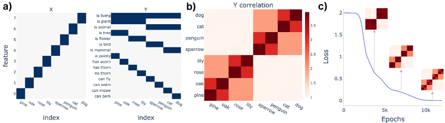
cat are all living animals, but ‘penguin’ is a bird and cat is a mammal. (b) The correlation matrix of the feature output shows a hierarchical structure. (c) The hierarchical structure is acquired progressively during the training of the deep linear neural network.Measuring influence dynamics.
First, we probe the local BIF (Kreer et al., 2025) on the toy model over the entire learning trajectory. We use RMSProp-preconditioned SGLD sampler introduced in Section 2.2 to estimate a posterior from each checkpoint at training time . See Appendix B for details of the local BIF implementation and Section C.2 for the hyperparameter sweep. Furthermore, we derive the dynamics of the influence function analytically, leveraging the mathematical tractability of the toy model (see Section C.6).
Leave-one-out (LOO) verification.
To confirm our observation from the BIF and analytical treatment, we conduct retraining experiments. Specifically, we consider the Leave-One-Out (LOO) setting, where we ablate one data point and measure the loss difference of other data points compared to the baseline loss without ablation. We measure the loss difference over training time :
| (3) |
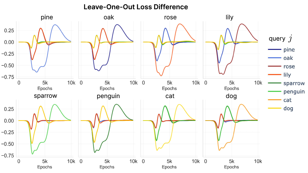
measured at time where is the full dataset, is the dataset with data index ablated, and is the index of the data point that we are querying. In Figure 3, we observe that the loss difference from LOO results in a similar pattern to what we see in the BIF and the analytical derivation, and validates their use. The additional results on perturbing other data points show consistent trend in Section C.2 and are also visible in the dampened classical IF Section C.4.
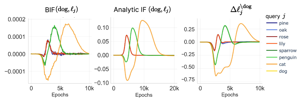
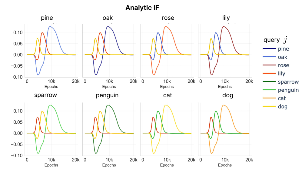
dog sample on other query samples with the following: (Left) BIF (). (Center) Analytical IF (see full derivation in Section C.6). (Right) Loss difference from Leave-One-Out (LOO) retraining experiment. All three measures agree that the influence one sample has on another can vary non-monotonically over the course of training as discussed in Section 3. See Section C.2 for additional pairs of samples and experimental details.With these results, we confirm the predictions from Section 2: (1) influence changes over time non-monotonically and can change sign, and (2) peaks in influence are correlated with key developmental transitions in model behavior. In the rest of the section, we will establish how these observations are reflected in the progressive learning of the hierarchical structure in our toy model.
“When” matters for measuring influence.
We clearly observe that influence goes through non-monotonic change over the course of training, strengthening our argument that a static interpretation of influence is fallacious. In Section C.6, we analytically derive that influence is a function of singular mode strength of data input-output covariance learned by the network, which is a time-dependent variable and thus justifies studying data attribution from a dynamic perspective. Over the course of training, each data point induces a non-static influence on other data points. The influence can flip sign—the same data can be either helpful or harmful, depending on when it is presented. It can also mark clear peaks at a specific time point on different query data points. Furthermore, the influence over time from one data point to another point is specific to those points. The influence from dog to cat might be the same as dog to ‘penguin’ early on, but they are distinguished later in the learning process. In Section C.5, we perform an additional retraining experiment showing that ablating data during the stage with the highest influence induces the largest loss difference.
Change of influence reflects stagewise learning.
During the phase where one hierarchical distinction (e.g., animal vs. plant) is being learned, upweighting a data point in the same class (dog) is helpful for learning a query data point (sparrow) as indicated by a negative influence (positive covariance). In contrast, upweighting a data point that belongs to a different class harms learning that query data point (pine), reflected in a positive influence. A data point dog is helpful (negative influence) to learning sparrow early on in the learning, while learning to distinguish animal vs. plant, but it is harmful (positive) later on when learning to distinguish mammal vs. bird. In Figure 4 b), we show Multi-Dimensional Scaling (MDS, Torgerson 1952; Cox & Cox 2008) of hidden representation of each data over time as in Saxe et al. (2019a) where learning of each hierarchical level is reflected on the branching node (numbered). We observe that the time point of the branching node matches the peaks in influence. That is, at the transition, where the model learns to distinguish mammal vs bird within the animals and form a new hierarchy level, the influence between mammal and bird is the highest.
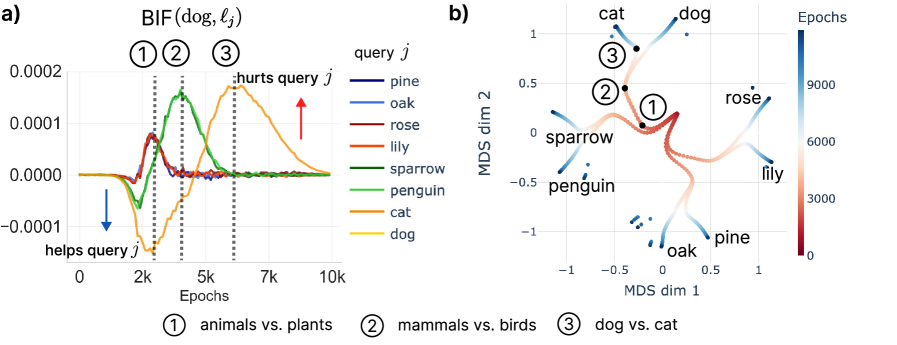
dog to different data points is noted with \raisebox{-0.9pt}{1}⃝, \raisebox{-0.9pt}{2}⃝, and \raisebox{-0.9pt}{3}⃝. (b) MDS of the hidden representations in the network over the course of learning. The peaks in influence match the branching points of the MDS trajectory, where each hierarchical category develops (black points).4 Language Models
To investigate the dynamics of influence in a real-world setting, we study the acquisition of token-level syntactic knowledge using language models from the Pythia Scaling Suite (Biderman et al., 2023).
We confirm our theoretical predictions in Section 2.3 by finding non-monotonic influence trajectories, with large changes in magnitude, sign flips, and peaks that correspond to known developmental changes like the formation of the induction circuit.
Per-token influence functions.
One clear benefit of the BIF in the language-modeling setting is that computing influence at the level of individual tokens rather than sequences incurs no additional computational cost. Loss is computed on a per-token basis during RMSprop-SGLD, which is already necessary when considering the autoregressive losses that represent the standard for LLM pretraining:
where is the th token in the th text sequence. These per-token losses can then be stored individually and used to estimate the per-token BIF matrix for the relevant dataset.
Classifying tokens into syntactic classes.
Following the experimental setup of Baker et al. (2025), we classify individual tokens according to how they are used to give structure to text. These classes include strictly syntactic tokens (left delimiters, right delimiters, and formatting tokens—such as newlines), morphological roles (parts of words and word endings), and a broader structural class—tokens that have been used in conjunction earlier in the context, forming an inductive pattern. We note that this classification is not exhaustive, nor is it exclusive—not all tokens have a class, and some may occupy multiple classes at once. A full classification is provided in Section D.1.1.
Calculating group influence.
To estimate patterns of influence between tokens across classes, we make use of the following procedure:
-
Using a subset of The Pile (Gao et al., 2021), we compute the normalized BIF (Kreer et al., 2025) between all pairs of tokens, sampled from the SGLD-estimated model posterior, as described in Algorithm 1.
-
Each token is classified in accordance with the listed structural classes based on pattern-matching, following Baker et al. (2025).
-
For every possible pair of classes, we compute the average (or “group”) influence between tokens in these classes, excluding influences between the same token in different classes.
These inter-class influences can then be used to provide insight into how much influence tokens from one class have tokens from other classes.
Learning induction.
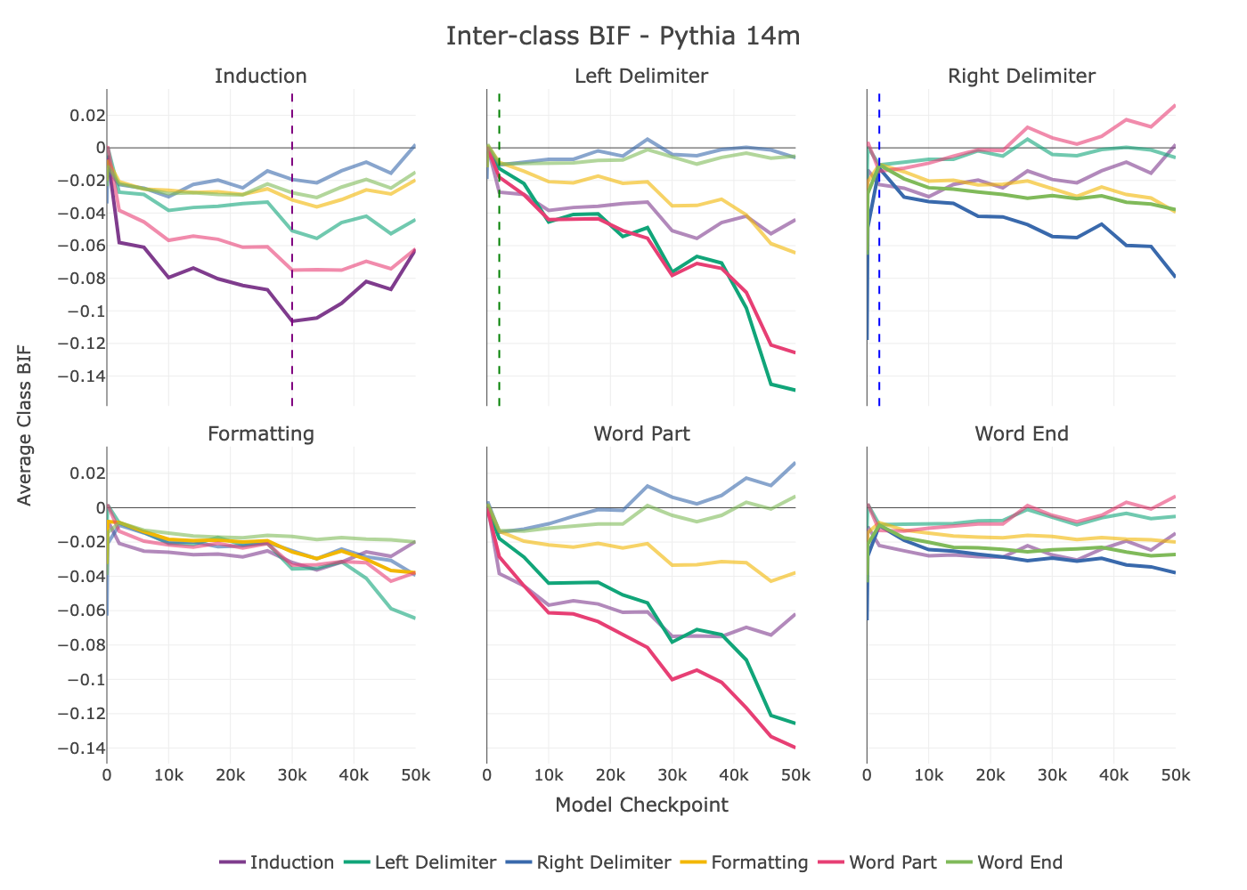
In Figure 5, we plot the inter-class influence for each query class across all class pairings at several model checkpoints. From these plots, some clear dynamics emerge. We see that the formation of model structures capturing induction relationships in the BIF starts as early as 1000 steps into learning, and continues to strengthen for the next 30k training steps before appearing to peak and fall, corresponding with the results of Tigges et al. (2024), which finds that Pythia models begin to learn the induction circuit at this time, and exhibit an apex at 30k training steps before diminishing. In Section D.2, we study a small language model trained from scratch and use influence patterns on a targeted set of synthetic samples to isolate this induction bump.
Learning where to end.
Another notable pattern occurs in the influence traces of left delimiters and right delimiters. Both classes appear among high-influence tokens for the other class very early in training, but this relationship quickly inverts, with tokens from the opposite delimiter class progressively becoming increasingly negative as the model learns to distinguish between these classes. We also see increasing influence between left and right delimiters and related classes that may perform similar roles in structuring text. Left delimiters share high influence with parts of words but not the ends of words, while right delimiters share uplifted influence with ends of words but not word parts. These relationships are also visible in the reverse direction (from word parts / word ends to left / right delimiters). These relationships develop over time, with a particularly notable spike in the relationship between word parts and left delimiters later in model training.
Dynamics of influence.
Taken together, these results demonstrate that influence between different classes of tokens is not a static property but a dynamic one that evolves throughout training. We observe changes in both the magnitude and sign of influence, with the timing of these shifts varying depending on the specific structural capability being learned. For instance, the influence related to induction patterns exhibits a non-monotonic peak that aligns with the known developmental phase transition for this circuit. Similarly, the relationship between left and right delimiters undergoes a sign flip, indicating a qualitative shift in how the model processes scope and pairing. These findings confirm the predictions of our stagewise framework: different data becomes influential at different times, reflecting the model’s progressive, stage-by-stage acquisition of syntactic and structural knowledge.
5 Discussion & Conclusion
Stagewise data attribution and developmental interpretability.
This work places data attribution within the context of Developmental Interpretability. We follow the established methodology of using singular learning theory (SLT) as a theoretical lens to study the dynamics of models trained with stochastic optimizers. Prior work has successfully used this pipeline to explain phenomena like phase transitions in toy models of superposition (Chen et al., 2023), algorithm selection in transformers (Carroll et al., 2025), stagewise learning in toy transformers (Urdshals & Urdshals, 2025), and the stagewise emergence of structure (e.g., n-grams, induction, parenthesis-matching, space-counting) in language models (Hoogland et al., 2024; Wang et al., 2025b; Baker et al., 2025; Wang et al., 2025a). Our contribution is to use the SLT account of phase transitions to predict and subsequently verify that a training sample’s influence is not static but a dynamic quantity that evolves with the model’s development.
Stagewise vs. unrolling-based attribution.
Our work complements another important line of research that moves beyond static influence functions: trajectory-based or “unrolling” methods like TracIn (Pruthi et al., 2020), HyDRA (Chen et al., 2021), and SOURCE (Bae et al., 2024). These techniques approximate the total influence of a sample by integrating its contributions (such as gradient updates or local influence scores) across numerous checkpoints along the full training path. This approach provides a more faithful account of the path-dependent nature of SGD and can offer more accurate attribution scores than single-point estimates.
However, the fundamental goal of these methods differs from ours. Unrolling techniques compute a single, cumulative score that summarizes a sample’s total impact over the entire trajectory. In doing so, they treat the learning process as a black box, rather than an object of study in itself.
A mechanism for implicit curricula.
The concept of a curriculum—learning from easier to harder data—has been argued consistently for more efficient neural learning (Bengio et al., 2009; Wang et al., 2021; Lee et al., 2024). However, the efficacy of this technique has been shown to be limited in practice (Wu et al., 2020; Mannelli et al., 2024). One prevalent explanation is that an implicit curriculum is adopted by learning through gradient descent in neural networks (Graves et al., 2017; Rahaman et al., 2019; Saxe et al., 2019a; Valle-Perez et al., 2018). Our findings provide a new, more granular mechanism for understanding this phenomenon. The stagewise evolution of influence demonstrates how different data points become “important” at different moments, effectively creating a dynamic, self-organizing curriculum.
Limitations and future work.
Our framework points toward several avenues for future research. The primary theoretical gap remains the link between the Bayesian learning process of SLT and the non-equilibrium dynamics of SGD. On the empirical front, a key direction is to move from a behavioral to a mechanistic account of influence. Ultimately, model generalization is grounded in the circuits and internal structure a model acquires over training. A more complete science of interpretability therefore understands not just which samples are most influential (data attribution), but when they are most influential (stagewise attribution), and how they shape model internals such as features and circuits (mechanistic interpretability).
From pointwise to stagewise data attribution.
Ultimately, this paper argues for a shift in how we approach training data attribution. The static perspective, which assigns a single, global influence score to each data point, only at the end of training, offers an incomplete and, at times, misleading picture. By demonstrating that influence is inseparable from development, we advocate for moving from point-wise to stagewise data attribution.
This developmental lens is essential for tackling a key scientific challenge: understanding the correspondence between data structure, loss landscape geometry, learning dynamics, and model internals (Wang et al., 2025b). Stagewise data attribution, by tracking influence dynamics, provide a concrete tool to map these connections, opening new possibilities for interpreting, debugging, and ultimately steering how models learn.
Appendix
-
Appendix A: Phase Transitions. This section provides a formal outline of how phase transitions arise in singular models and how they impact influence functions.
-
Appendix B: Bayesian Influence Functions. This section provides additional experimental details on estimating the local BIF.
-
Appendix C: Toy Model Details and Additional Results. This subsection describes the hierarchical dataset, model architecture, and Leave-One-Out (LOO) training procedure. It also contains additional LOO results and the full analytical derivation of the influence dynamics in the deep linear network model.
-
Appendix D: Language Model Details and Additional Results. This subsection describes the structural token classification scheme, provides RMSPropSGLD hyperparameters for the Pythia experiments, and details additional validation experiments.
Appendix A Phase Transitions
In this appendix, we provide a theoretical justification for the claims made in Section 2 regarding phase transitions and their effect on model predictions and influence, grounded in statistical physics and the theory of Bayesian statistics. This theoretical treatment motivates our empirical investigation into the interaction between stagewise development and influence functions for models trained via standard stochastic optimizers.
A.1 BIF as Susceptibility
Setup.
We begin with the model-truth-prior triplet:
-
The model assigns a probability to a sample for a given choice of weights .
-
The truth or data-generating distribution generates a dataset of i.i.d. samples .
-
The prior assigns an initial probability distribution to each choice of weights.
From this triplet, we obtain a posterior through (the repeated application of) Bayes’ rules:
| (4) |
where is the likelihood, and is the marginal likelihood. Often, we’re interested in a tempered Bayesian posterior:
| (5) |
where is a vector of per-sample importance weights, and is the vector of per-sample losses for a given weight .
The (global) free energy formula.
The (global) free energy is the negative log marginal likelihood, . A central result of singular learning theory (SLT; Watanabe 2009) is an asymptotic (in the limit of infinite data) expression for this quantity. For a critical point in a neighborhood , the free energy asymptotically expands as
| (6) |
where is the learning coefficient, a degeneracy-aware measure of complexity (that coincides with half the effective parameter count for minimally singular models).
Free energy as moment-generating function.
In statistical physics and thermodynamics, the free energy is the central object of study. This is because, if one manages to obtain a closed-form expression for the free energy, it is possible to calculate arbitrary expectation values simply by differentiating the free energy. Expectation values are of primary interest because they correspond to the things we can measure in an experimental setting.
For example, in the learning theory setting, the expected (per-sample) loss can be expressed as
| (7) |
Combining Equation 7 with Equation 2, lets us express the BIF as a 2nd-order derivative of the free energy, assuming both samples are in the training dataset:
| (8) |
Susceptibilities are defined as second-order derivatives of the free energy, which makes the BIF an example of a generalized susceptibility.
A.2 Internal Model Selection
The (local) free energy formula.
The local free energy formula is defined analogously to the global free energy, but with the domain of integration restricted to a particular region of parameter space or “phase” :
| (9) |
This admits an analogous asymptotic form to Equation 6:
| (10) |
but where now is a local minimum within , and is the local learning coefficient associated with that local minimum (Lau et al., 2025).
Coarse-graining.
Given a partitioning of parameter space into multiple disjoint “phases” , the global free energy can be computed from the local per-phase free energies as follows:
| (11) | ||||
| (12) | ||||
| (13) | ||||
| (14) |
The last line follows from the well-known use of a log-sum exponential as a smooth approximation for the max function. This is to say that globally, the free energy is determined primarily by the phase with the lowest free energy, with exponentially suppressed contributions from all other regions of phase space.
Competition between phases.
Assume the posterior distribution is concentrated in just two distinct neighborhoods, which we label and , and is vanishing everywhere else. That is, these two phases constitute a degenerate set of minimizers of the free energy. We can then write the posterior as a mixture distribution:
where is the posterior distribution conditioned on the model being in phase , and is the total posterior probability of this phase, with .
First-order phase transitions.
This free energy formula predicts the existence of first-order “Bayesian” phase transitions. When two solutions compete, e.g., with neighborhood and with neighborhood , then the posterior log-odds evolve as , where and . If has higher loss but lower complexity (, ), the posterior initially prefers the simple solution but switches to the complex solution when . This is a “Type-A” transition (Carroll et al., 2025; Hoogland et al., 2025), see Figure 1.
Alternatively, if the two phases agree on the linear term (they have the same minimum loss), then the trade-off will be pushed down into lower-order terms, and there can be a “Type-B” transition, in which complexity (as measured by the LLC) decreases, in exchange for an increase in lower-order terms.
Appendix B Bayesian Influence Functions
Estimating the BIF with SGMCMC.
To estimate the BIF in practice, we use an RMSProp-preconditioned SGLD sampler (Welling & Teh, 2011; Li et al., 2016) to estimate a posterior from each checkpoint This approximates Langevin dynamics with loss gradients and locality regularization from initial modulated by localization strength ,
| (15) |
The update rule takes advantage of an adaptive learning rate compared to vanilla SGLD and is more robust to varying step size (Hitchcock et al., 2025). The full algorithm is described in Algorithm 1.
Practical considerations with the BIF.
As mentioned in the main body and following the discussion at length in Kreer et al. (2025), we consider several practical modification of the local BIF. First, we use a normalized BIF for the language-modeling experiments, which involves computing the Pearson correlation instead of the covariance over losses. Empirically, we find that this behaves more stably than the raw covariance and thus is easier to track over time. Second, we consider a per-token BIF, which can be trivially obtained by avoiding the loss accumulation over token indices and saving all per-token losses at each SGLD draw. Finally, to avoid potentially spuriously high covariances, we drop same-token influence scores when computing aggregate group influence scores, as in Adam et al. (2025).
Addressing influence from unseen training samples.
A potential objection to our developmental analysis is that at early checkpoints, the model’s optimizer has not yet encountered every training sample. It might therefore seem paradoxical to measure the “influence” of a sample the model has not yet “seen.”
This concern can be straightforwardly resolved. The BIF is defined as the sensitivity of an observable to a sample’s contribution weight, , to the total loss. For a sample that has already been processed, we measure influence by considering perturbations around its baseline weight of . For a sample the optimizer has not yet encountered, we can simply treat its current weight as and evaluate the same derivative at that point.
The resulting quantity remains well-defined, with a slightly different interpretation: it measures the model’s sensitivity to the initial introduction of a new sample, rather than the re-weighting of an existing one. Our practical implementation naturally accommodates this, as we use independent data sources for the SGLD gradient updates and the forward passes used to compute the loss covariance.
Appendix C Toy Model of Development
In this section, we provide details of the toy model experimental details and analytical investigation of deep linear neural network learning dynamics under the data perturbation introduced in Section 3. It includes a training setup of toy data with a 2-layer deep linear neural network and BIF hyperparameter sweeps, and extended results of the Leave-One-Out (LOO) experiments and BIF measurements.
C.1 Toy Dataset
We use the semantic hierarchical dataset introduced in Saxe et al. (2019a). We set the number of data points with hierarchy level , that is, the data can be organized by 4 levels of hierarchy, e.g., dog belongs to the lowest hierarchy level 1 of living organism, and level 2 of animals (vs. plants), and level 3 of mammals (vs. birds). The input is a data index given by an identity matrix of size . The model needs to learn to associate with the feature of each data point, which forms the above hierarchical structure, the output size of with .
We train a 2-layer bias-free linear neural network with 50 hidden neurons, which is overparameterized for our rank 8 dataset. We initialize the network with small weights by sampling from a Gaussian distribution . We train the network on mean squared error (MSE) loss with a small learning rate and train for epochs with full batch unless mentioned otherwise.
C.2 BIF Additional Results and Hyperparameters Sweep
For a principled decision of hyperparameters for the SGLD sampler, we perform a preliminary hyperparameter sweep on the SGLD sampler using the same deep linear neural network architecture and the data to estimate LLC. Since ground truth LLC is known for deep linear neural networks (Aoyagi, 2024), we can select a range of hyperparameters by choosing ones that have a well-matched LLC estimate to the ground truth. Based on this procedure, we validate the superiority of RMSPropSGLD to vanilla SGLD and also the insensitivity of the sampler quality to decay rate and stability constant in a certain range and fixed the value to reduce the grid search dimension. We also narrowed down the localization strength range.
The range of the conducted hyperparameter sweeps for BIF measurement is summarized in Table 1. The values given in the range were sampled on a logarithmic scale. RMSPropSGLD sampling procedure is shown in 1.
| Hyperparameter | Range |
|---|---|
| (step size) | [1e-7 - 1e-2] |
| (inverse temperature) | [1e+1 - 1e+4] |
| (localization strength) | [1e-2 - 1e+6] |
| (batch size) | 8 (full batch) |
| (number of chains) | [2,4,8] |
| (chain length) | [200, 400, 800, 1000] |
| (decay rate) | [0.8, 0.9, 0.95, 0.99] |
| (stability constant) | [1e-4 - 1.0] |
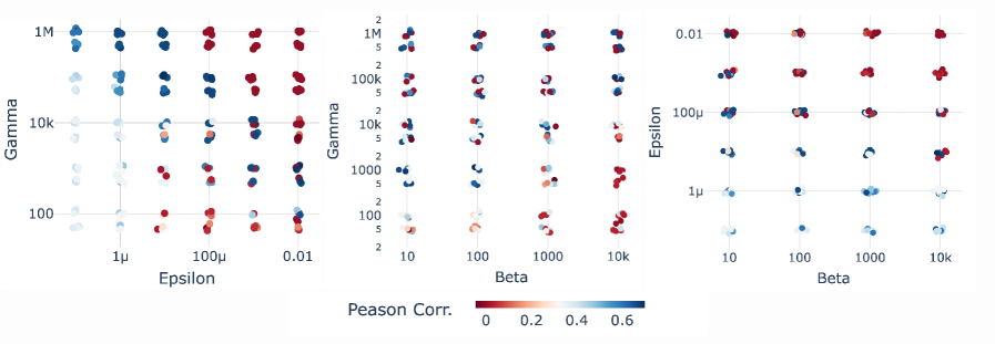
We present the Pearson correlation coefficient between Leave-One-Out (LOO) loss difference trajectory and BIF trajectory over learning over varying hyperparameter choices of inverse temperature , localization strength and step size in Figure 6. In Figure 6, we see that the correlation coefficient changes smoothly as we vary the hyperparameters. In the main Section 3 Figure 3, we showed the BIF measured with the hyperparameters that have the highest correlation with LOO ().
C.3 Leave-One-Out (LOO) Experiment
For the Leave-One-Out (LOO) experiment, which is also referred to as retraining, we mask the corresponding data index to 0 for both input and output. We use the same hyperparameter as above and we report the loss difference of data after ablating data at each time, .

C.4 Classical Influence Function
We measure classical influence over the training trajectory of the toy model
| (16) |
at time . Note that we do not use the global minimum but the minimum at that specific measurement time . Since the Hessian of the overparameterized neural network is non-invertible due to multiple zero / near-zero eigenvalues, we take the approximation methods as in Koh & Liang (2020); Grosse et al. (2023). First is to add a constant dampening term to the Hessian,
| (17) |
Suitable enforces to have positive eigenvalues. Grosse et al. (2023); Martens & Grosse (2015); Bae et al. (2022) used damped Gauss-Newton-Hessian (GNH), an approximation to which linearizes the network’s parameter-output mapping around the current parameters,
| (18) | |||
| (19) |
Using approximated damped-Hessian () and damped GNH (, we measure classical influence function over time (Eq. eq:cif-time) with varying dampening constant .
The dampening constant is scaled with , the maximum absolute value of all eigenvalues of the
| (20) |
and we vary in range of in logarithmic scale.
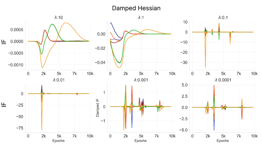
dog sample with damped Hessian approximation with varying dampening constant .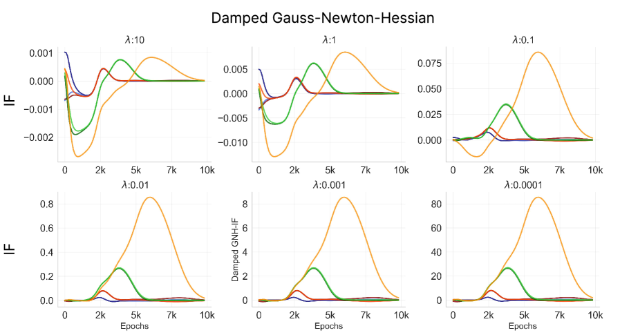
dog sample with damped Gauss-Newton-Hessian approximation with varying dampening constant .C.5 Time-Specific Ablation Experiment
Our observation that influence is a time-dependent function proposes another perspective - perturbing the same data point but at different training times would lead to non-identical influence. That is, the exact moment the network interacts with each data point matters. Here we probe this hypothesis with a simple retraining experiment in the toy model. We hypothesize that the measured influence trajectory tells us which time point would be most critical for a model to learning each sample. For example, the influence of dog on cat makes a peak around , which implies ablating dog around that time would be most helpful in learning cat. We probe this hypothesis with a retraining experiment with a brief ablation at different stages of learning.
In Figure 11, we ablate a data point dog during the duration of epochs from and show the integrated loss difference compared to the baseline (no ablation) during . As we expected, the loss difference is the biggest around , when the highest influence occurs, indicating ablating dog was helpful the most at this stage. Similarly, we observe the negative peak of integrated loss difference around , which also matches the negative minimum in the influence measurement, implying that learning of the cat was the most detrimental at this time point when dog is ablated. We show that the most important stage changes with the query data that belongs to a different hierarchy, e.g., sparrow. Collectively, we strengthen our claim that influence over time shows us how a sample interacts with “what” data “when”, and that it is often correlated with the structure of the data, such as hierarchy.
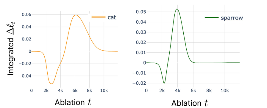
dog. For each experiment, we ablate dog for duration epochs starting from timepoint . Starting time is sampled uniformly with an interval of 200 epochs. For each experiment, we integrate the loss difference to the baseline during . We show the integrated loss of query (a) cat and (b) sparrow over different ablation windows. The most critical period of influence from the dog on the two samples is different. The higher level hierarchy (animals) sharing sample sparrow has an earlier critical point than the lower level hierarchy (mammals) sharing sample cat. C.6 Analytical Investigation of Toy Model
In this section, we analytically derive the dynamics of the influence function in a deep linear neural network. First, we introduce deep linear neural network learning dynamics studied in Saxe et al. (2013; 2019b) and then we show the time dependency of the influence function and its relation to progressive learning of the hierarchical structure.
Deep Linear Neural Network Learning Dynamics
Following the singular modes learning formulation in Saxe et al. (2019a; 2013), we can describe each data point ’s loss into the singular modes basis. We assume whitened input , and output . The input-output correlation and its singular value decomposition (SVD) become
| (21) | |||
| (22) |
With squared error loss, individual data point at data is . We project data to space (object analyzer) and its component becomes , where is a column vector of . Similarly, we project and with rank ,
| (23) |
is a singular mode strength of mode of the network obtained from
| (24) |
assuming the network and the data shares the aligned right and left singular vectors . This assumption holds with small initialization and small learning rate.
Now, we can compute the loss gradient with respect to the parameter space and decoupled mode space. In parameter space,
| (25) | |||
| (26) |
We can substitute the terms in singular decomposed form,
| (27) | |||
| (28) | |||
| (29) |
The effective singular values from each layer are and , which eventually aligns the effective weights’ singular vectors to that of the data correlation . In general, we cannot assume throughout learning, but the equality holds with the strictly balanced initialization. With the small initialization assumption, the first-order approximation of equality holds, which eventually allows us to write down the effective singular value trajectory throughout learning as in Saxe et al. (2019a).
Importantly, is a time-varying variable, evolving throughout the training that could be written in closed form with being corresponding diagonal singular value of from data covaraince,
| (30) |
and the model that learned the training data recovers
| (31) |
For convenience, we will drop the notation of time dependence in the rest of this section. For an end-to-end linear map define its representation in the data singular basis and the singular mode strength ,
| (32) |
For a data point write the coordinates in the original basis
| (33) |
the per-sample residual in mode space
| (34) |
and the per-sample loss gradient in mode space
| (35) |
Influence Function in Toy Model Using Single data point Perturbation
Following Cook & Weisberg (1982); Koh & Liang (2020), we will derive influence function, that is, the change in model prediction with a targeted perturbation of training data. In the following, we will derive the response of original and as a function of a single data point perturbation to derive the influence function in singular basis. With those in hand, we can use the closed-form dynamics on Eq. 30 to get time-dependent dynamics.
First, we consider a perturbation by upweighting a single data point with factor . The perturbed cross-covariance becomes
| (36) |
Let be the first-order derivative of the data covariance with upweighting of a single data point ,
| (37) |
With the perturbed dataset, the learned 2-layer linear network mapping at time becomes
| (38) | |||
| (39) |
where is a singular value from diagonals of and follows a closed form dynamics as given in Eq. 30. We assume that the network will have aligned singular basis with the perturbed data covariance, given in and . For convenience, we will move the parameter to a subscript and drop the perturbed data index .
We apply product rule to ,
| (40) |
We project the above perturbation to the singular mode coordinates,
| (41) |
Since are orthonormal matrices,
| (42) |
and differentiating these orthonormality constraints with respect to the perturbation
| (43) | |||
| (44) |
Due to orthonormality, lie in the tangent space of . We can define
| (45) |
where the orthonormal constraints give
| (46) |
and , become skew-symmetric, . Intuitively, is equivalent to the in-subspace angular velocity (rotation rate) of the columns of and due to the perturbation, respectively.
Now, we solve Eq. 47 for and . First, we consider a case where the singular values are non-degenerate. Due to the diagonal constraint of singular values, the response from the perturbation should also be diagonal for the singular values
| (48) |
The response of the singular basis is obtained from Eq. 45,
| (49) |
where
| (50) | |||
| (51) |
When has degenerate singular values or a near-zero gap, above is ill-defined as the denominator . In this case, we apply block perturbation, treating the whole invariant subspace (sharing the degenerate singular values) all at once.
We take the sets of the degenerate singular values , define the block coupling by projecting the perturbation on this block,
| (52) |
where and are sets of the degenerate singular values corresponding to sets of columns of and . It can be further decomposed into a symmetric and a symmetric-skewed part,
| (53) |
Due to diagonality constraints of singular values and zero-diagonals in the skew-symmetric part , the first-order singular value consistency reduces to . To have diagonal singular value matrix , we choose such that
| (54) |
where becomes the first-order splits within the degenerate block with preferred direction defined by . Skewed part sets the in-block angular velocity,
| (55) |
Then,
| (56) |
Now we are equipped with described by original we define influence on from the perturbation on a data point at fixed time by applying derivative on Eq. 38,
| (57) | |||
| (58) |
We can further derive influence on measurable in singular basis using the chain rule,
| (59) |
where is a squared loss of data point and is the perturbed data point. This perturbation is expected to hold with a small perturbation . We use down-weighting to approximate the ablation effect in Figure 3.
Appendix D Language Models
This section discusses additional experimental details for the language model experiments.
D.1 Structural Token Classification
Here, we present additional details and further experiments conducted to investigate the development of influence with respect to how tokens structure text. These experiments were conducted using the 14 million parameter Pythia model. Tokens are generated using the same tokenizer as the Pythia models use in order to be able to use these tokens with the model suite.
D.1.1 Token Classes
Tokens are classified based on their role in structuring text. The classes we used are based on the classes used by Baker et al. (2025). Figure 13 demonstrates these classes graphically, with tokens outlined in bold indicating class membership, and distinct colors representing distinct classes.
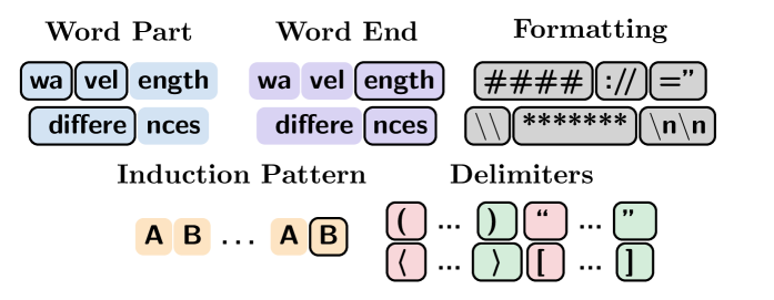
The classes are as follows:
- Word Part
-
Tokens that constitute a part of a word that is not the end of the word. This class excludes tokens that represent entire words or entire words with the addition of additional characters (e.g. a space and an entire word).
- Word End
-
Tokens that constitute the ending of a multi-token word. This class also excludes tokens that represent entire words and entire words with the addition of additional characters.
- Formatting
-
Tokens that are generally used to format text including newlines and repeated characters.
- Induction Pattern
-
Tokens that appear in a context in which the token is preceded by another particular token, and the same token has been preceded by the same other token earlier in the context.
- Left Delimiters
-
Tokens that are generally eventually followed by an equivalent right delimiter with interceding text generally considered to occupy a distinct scope.
- Right Delimiters
-
Tokens that close the scope opened by a paired left delimiter.
D.1.2 RMSPropSGLD Hyperparameters
| Hyperparameter | Range |
|---|---|
| (number of sequences) | |
| (sequence length) | |
| (step size) | |
| (inverse temperature) | |
| (localization strength) | |
| (batch size) | |
| (number of chains) | |
| (chain length) | |
| burn in steps | |
| (nearest neighbors) |
We found that the overall dynamics expressed by the BIF did not vary substantially among hyperparameters chosen in this setting. Plots in the main paper were selected based on the parameters that optimized the average class recall on the KNN experiment which is discussed in section Section D.1.3
D.1.3 Same-class prediction with BIF K-Nearest Neighbors
One way to investigate the ability of the BIF to capture what sorts of text structure a model has learned is to use it to predict which structural class a token belongs to based on the classes that token shares high influence with.
We query the predictive capacity of token-level influences using a simple nearest-neighbors approach. The predictive model is as follows:
where is the indicator function for elements of class , and is the token-dependent class frequency in the dataset:
with denoting the set of all tokens that are not . Tokens are thus predicted to have the majority label of their corresponding top-influence set , adjusted for class rates overall.
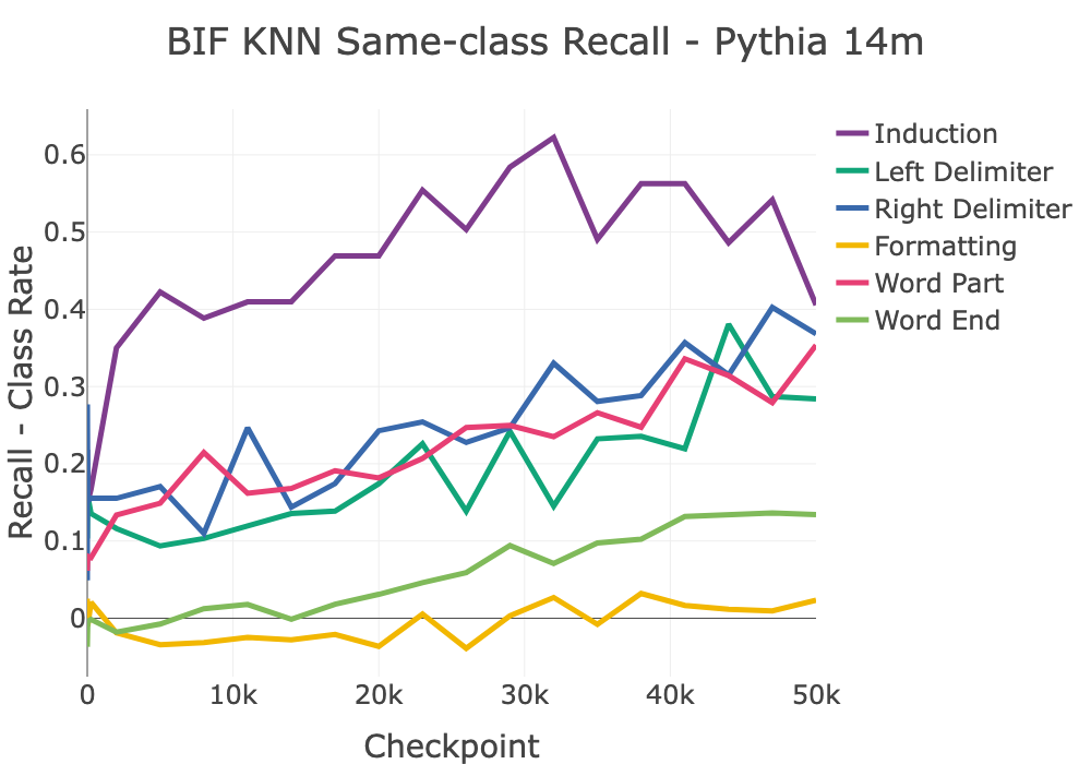
Figure 14 shows the results of this experiment. We observe that the classes of high-influence other tokens act as a better than random predictor for all classes by the end of training, with recall generally improving as the model progresses through training.
D.2 Learning Induction
Our initial experiments with the public Pythia checkpoints (Biderman et al., 2023) suggest a signal for the learning of induction patterns. However, the checkpoint frequency was too coarse in the vicinity of checkpoints 1k to 10k to observe the fine-grained dynamics of this developmental transition. To investigate this critical phase in more detail, we trained a Pythia-14M model from scratch, saving checkpoints every 100 steps for the first 20,000 training steps. Though we train on the same Pile data (Gao et al., 2021), it is in a different order and on different hardware, which means this training run is not the same as the original Pythia-14M training run.
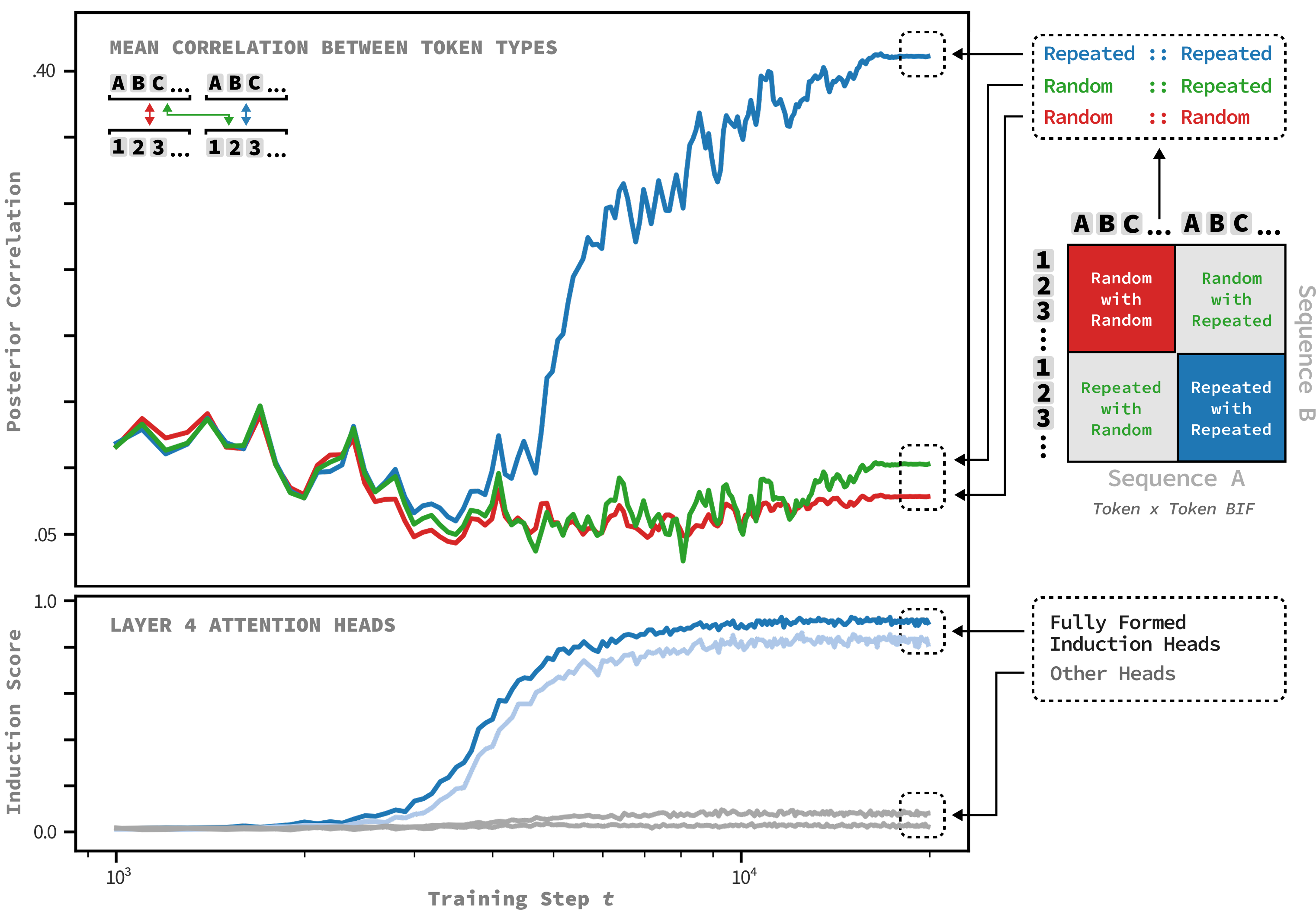
We constructed a synthetic dataset with sequences where the second half repeats the first, e.g., Sequence 1: A B A B and Sequence 2: C D C D. Sequences were constructed as to not share tokens. The first half of each sequence is made up of random tokens, and so the only structure that can be used for prediction is the repetition of the second half of the context.
During SGLD we collect losses on this dataset, but sample using the Pile, meaning that loss on these synthetic samples does not affect our sampling trajectory. We compute the BIF matrices at each checkpoint of our homemade Pythia-14M and then look at the mean correlation between the different parts of our sequence (Namely repeated tokens with repeated tokens from other sequences, non-repeated tokens with non-repeated tokens from other sequences, and non-repeated tokens with repeated tokens from other sequences).
The results are shown in Figure 15. The influence between tokens in the repeated segments of each sequence (top panel, blue line) undergoes a sudden, large increase, peaking and then stabilizing. Meanwhile, the BIF between non-repeated segments or across non-repeated and repeated segments shows no such change.
Simultaneously, we measure the “induction score” of the model’s attention heads—a standard metric from mechanistic interpretability that quantifies how strongly a head implements the induction algorithm (Olsson et al., 2022). As shown in the bottom panel, the induction score for the heads that become the “induction heads” begins to rise right before the BIF increases between the repeated groups.
Cite as
@article{lee2025influence,
  author = {Jin Hwa Lee and Matthew Smith and Maxwell Adam and Jesse Hoogland},
  title = {Influence Dynamics and Stagewise Data Attribution},
  year = {2025},
  url = {https://arxiv.org/abs/2510.12071},
  eprint = {2510.12071},
  archivePrefix = {arXiv},
  abstract = {Current training data attribution (TDA) methods treat the influence one sample has on another as static, but neural networks learn in distinct stages that exhibit changing patterns of influence. In this work, we introduce a framework for stagewise data attribution grounded in singular learning theory. We predict that influence can change non-monotonically, including sign flips and sharp peaks at developmental transitions. We first validate these predictions analytically and empirically in a toy model, showing that dynamic shifts in influence directly map to the model's progressive learning of a semantic hierarchy. Finally, we demonstrate these phenomena at scale in language models, where token-level influence changes align with known developmental stages.}
}