Section 1

Background and Motivation

Section 2

Polygons and Phases

Section 3

Susceptibilities and Patterning

Section 4

Test in the Small, Push in the Large

Section 5

A Local Theory of Polygon Phase Transitions

Section 6

Crafting Gons

Section 7

Rewriting Minima

Section 8

Trajectories in the Space of Data Distributions

Section 9

Patterning on the Loss

Section 10

Computing Susceptibilities at and around Singularities

Section 11

Patterning as Control

Section 12

Discussion, Related work, and Outlook

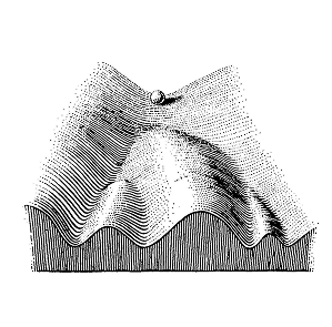
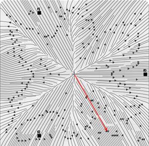
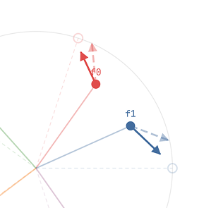
Reading: from** developmental biology to developmental interpretability.** In 1957, Conrad Waddington proposed the epigenetic landscape as an analogy for cell differentiation. Picture a marble at the top of a hillside carved with branching valleys. At each fork the cell commits to one developmental path or another. The final resting place determines what kind of cell it has become.

Neural networks develop in a comparable way. Training is the marble’s descent, here rolling down a landscape carved by the loss. Through a series of transitions, the model commits to one internal structure over other potential structuresanother. These transitions dictate the ways in which the model will generalize.

The developmental perspective gives biologists enormous leverage: instead of cataloguing every adult cell by its full transcriptome, they trace it back to a handful of commitment events on a lineage tree. Developmental interpretability (hoogland2025) pursues an analogous move for neural networks — read internal structure in trained networks by characterizing the developmental stages that produced it.

Writing:** from interpretability to patterning. **Models today are grown, not programmed: we pick a loss and a dataset, and the model’s structure is whatever training produces. Developmental interpretability lets us read what we got. But reading doesn’t let us change anything — for that we need to write. The goal is models that are crafted, not grown.

“Patterning” is our answer to what it means to “write” neural networks. Patterning works by minimising the loss, subject to constraints on posterior expectation values. That is, we want low loss, but also the ability to select among the many possible ways of realising that loss. By doing so we are able to .

Methodologically we combine two ideas: first, measure internal structure not by point evaluations but by expectation values averaged over the local loss landscape. This is what we call “spectroscopy,” following the tradition of statistical physics. Second, optimize not just over model parameters but also over the data mixture, using the derivatives of these expectation values to compute which data changes produce which structural changes. This is control in the precise sense: a feedback loop connecting data interventions to structural outcomes, and so can be naturally studied through the lens of control theory.

In this post, we demonstrate patterning in Anthropic’s Toy Models of Superposition (TMS)—a deliberately simple setting where internal structure is immediately visible. In this setting, we show:

1. Patterning allows choosing between developmental branches. Ordinary training commits to a branch at random. Via patterning, we are able to perfectly control these crucial developmental moments.
2. Patterning allows moving a trained model between solutions. We show that patterning can move a model at a global minimum between equivalent but disconnected solutions, crossing loss barriers that gradient descent cannot.
3. Patterning works where classical methods don’t. We show that at the bifurcation points—where control matters most—influence functions and second-order methods get no signal. Patterning finds its signal in the higher-order geometry these methods miss.

Toy Models of Superposition

We begin with a recap of the toy model of superposition (Section 2.1; Elhage et al. (2022)), define “internal structure” for this model (Section 2.2), and describe the model’s stagewise development (Section 2.3).

The Model

Anthropic’s Toy Models of Superposition (Elhage et al. 2022) introduced a minimal setting for studying superposition, the phenomenon where neural networks represent more features than they have dimensions. This motivated a subsequent line of work that culminated in sparse autoencoders, which occupy a central role in mainstream mechanistic interpretability (bricken2023).

We study the same model but for different reasons: First, its internal structure is visible in two dimensions, making it easy to just “see” the structure of the model. Second, the model exhibits clear developmental stages, with equivalent solutions chosen between at each transition. This makes it a clean instance of the kind of structural choice that we expect to find, in more complex forms, in larger models.

Following Elhage et al. (2022), we consider a tiny ReLU autoencoder (without a bias for simplicity). Inputs are binary feature vectors $x \in {0,1}^d$ drawn from a distribution $q$, in which each feature is active with an independent probability $p=1-S$, where $S$ is the “sparsity”. The model learns a feature dictionary $W \in \mathbb{R}^{m \times d}$ with representation $r = \mathrm{ReLU}(W x)$ and reconstruction $\hat{x} = W^T r$. We train against the feature-weighted MSE,

$$L = \sum_x \sum_i I_i (x_i - \hat{x}_i)^2,$$

where $I_i$ is the feature importance. By default, we focus on the uniform importance ($I_i=1$) regime.

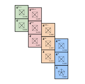
In the high-sparsity regime, learned feature vectors arrange into a polygonal geometry: $d$ features in a 2D hidden space form a regular $d$-gon when optimally packed. In this work, we focus on $d=5$.

Digon

Triangle

Square

Pentagon

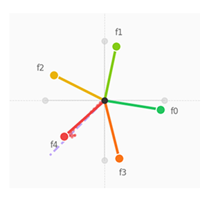
Because the encoder matrix $W$ has shape $(d, 2)$, each feature’s hidden representation is a two dimensional vector, which allows for easy visualization. The above figure shows the ideal digon, triangle, square, and pentagon forms of the model.

$W$ contains more information than just the polygon’s shape: rotating all feature vectors by the same angle gives a completely different $W$ with identical behavior and loss, making the absolute orientation a redundant degree of freedom. There are also discrete symmetries. Under uniform importance, the polygon has a $D_5$ symmetry: permuting the feature labels or reflecting the polygon leaves the loss unchanged. These symmetries break when features have different importances or correlated sparsity patterns. For example, features that co-occur frequently tend to be represented orthogonally when possible and side by side when not (Elhage et al. 2022).

Defining Structure

Patterning targets structure. So we need a language for describing structure. Here we borrow our first concept from statistical physics, and define an appropriate set of observables: functions $\phi_i(w): \mathcal{W} \to \mathbb{R}$ that map a model’s parameters to real numbers. An observable is “right” when it captures a degree of freedom that matters for distinguishing model behavior while discarding the degrees of freedom that don’t.

The structure of the toy model of superposition is simple enough that we can write down the right observables by hand. In general, this is a deep and central problem; we return to it in the discussion.

We define two sets of observables:

$\phi_{\text{dot}[i,j]} = W_i \!\cdot\! W_j / |W_i||W_j|$

(Normalized) Dot products measure angles between feature pairs. For a regular $n$-gon, adjacent features have dot product $\cos(2\pi/n)$.

$\phi_{\text{norm}[i]}(W) = |W_i|$

Norms measure feature magnitude.

Together, these 15 observables (10 dot products + 5 norms, for our 5-feature model) form a coordinate system over possible structures. A particular set of values is a “macrostate” in the language of statistical physics. This is the level of description at which we will define targets, measure responses, and steer development.

Stagewise Development

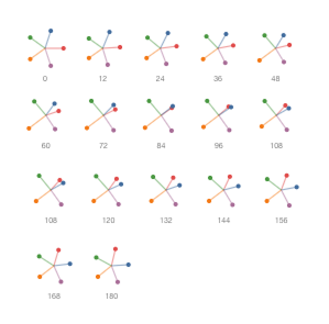
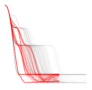
Training from a small, random initialization, the model usually passes through some sequence of polygon phases: 2-gon (antipodal pair), 3-gon (triangle), 4-gon (square), and so on, with each stage separated by discrete jumps. As in biological systems, the model develops in stages from simple, undifferentiated states to progressively more complex and specialized states.

Singular learning theory (SLT) provides a framework for understanding this (watanabe2009algebraic). chen2023 showed that each polygon is a critical point of the loss, characterized by its loss together with its local learning coefficient $\lambda$—a geometric invariant measuring the ‘degeneracy’ or ‘complexity’ of the critical point. Early in training, the posterior concentrates on low-$\lambda$ (simple) solutions despite their higher loss. As training progresses, it shifts toward low-loss solutions with higher $\lambda$.

SLT analysis of TMS following chen2023

Why does the model develop through polygon phases in order, rather than jumping straight to the best solution?

SLT provides an answer but this comes with a caveat: SLT is a theory of Bayesian learning, not of SGD-based learning. That is, SLT describes how the posterior over parameters evolves as the dataset size $n$ grows, not how the distribution of parameters obtained by SGD varies with training time $t$.

The basic idea behind developmental interpretability (devinterp, Wang et al. (2025)) is to treat the Bayesian account as an idealized model of learning by SGD and thus to use SLT to analyze real-world training. chen2023 showed empirically that this idealization works well in the TMS setting: the transitions predicted by the Bayesian theory occur in the same order during SGD training, and the LLC tracks the complexity of the polygon phase the model occupies.

Making rigorous connections between these learning paradigms is an active area of research and one we expect will close in the future. But, for the moment, the empirical justification from chen2023 will suffice. We now give the Bayesian account of TMS.

A key result of SLT is the asymptotic expansion of the free energy of a region $\mathcal{U}$ around a local minimum $w^*$:

$F_n(\mathcal{U}) = n L_n(w^*) + \lambda(w^*) \log n + O_p(\log\log n),$

where $\lambda(w^*)$ is the local learning coefficient and $n$ is the dataset size. The free energy governs how much posterior mass concentrates in each region. When two solutions $A$ and $B$ compete, the log posterior odds is

$\log \frac{p_n(\mathcal{U}_A)}{p_n(\mathcal{U}_B)} = n \Delta L + \Delta\lambda \cdot \log n + \ldots$

The first term favors lower loss; the second favors lower $\lambda$ (simpler geometry). At small $n$, the $\lambda \log n$ term dominates, so the posterior concentrates on simple solutions despite their higher loss. As $n$ grows, the $n \Delta L$ term wins and the posterior shifts to the lower-loss, more complex solution. This crossover is a Bayesian phase transition.

This is the process of internal model selection (watanabe2009, chen2023): Bayesian inference performs an automatic tradeoff between accuracy and complexity, with the LLC playing the role that parameter count plays in the BIC for regular models. In TMS, each $n$-gon is a critical point with a characteristic loss and LLC. The 2-gon has the lowest $\lambda$ but highest loss. The 5-gon has the highest $\lambda$ but lowest loss. Training replays this tradeoff, producing the characteristic staircase in both loss and LLC.

Note that the Bayesian transition described here is first-order: the posterior mass shifts discretely between competing basins as $n$ crosses a critical threshold. Later in this post, we analyze the 4-to-5-gon bifurcation as a second-order transition: the dead feature grows continuously from zero through a quartic potential, with diverging susceptibility at the critical point. These two pictures may not be as in conflict as they appear to be, but reconciling them is beyond the present scope, and we leave it to future work.

Read more about the SLT account of TMS here.

Loading...

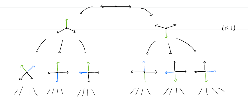
Development is stochastic: at each transition, the model can proceed down multiple possible paths. A symmetric $n$-gon has $n$ equivalent ways to become an $(n+1)$-gon, corresponding to the $n$ gaps between features. In ordinary training, noise breaks the symmetry and picks one branch randomly.

In biological development, there is an analogous problem with cell differentiation, where cells must “choose” between different possible cell fates. But unlike in deep learning, these choices are tightly controlled by the organism. This is accomplished via morphogens: signaling molecules that form concentration gradients across fields of otherwise identical cells. In Wolpert’s French flag model, a single morphogen gradient is sufficient to produce three distinct cell fates from a uniform population. Cells exposed to high concentrations adopt one fate, cells at medium concentrations another, and cells at low concentrations a third. The morphogen doesn’t build anything directly. It biases which of several otherwise equivalent developmental paths each cell takes.

[French flag / TMS patterning figure]

Through patterning, we will show that we can achieve the same kind of control over TMS development, simply by reweighting the training data mixture. Like a morphogen gradient, this is an external signal that doesn’t intervene on the model’s internal weights directly. Instead, it biases the learning dynamics toward specific outcomes. In Section TODO, we show how to compute the right reweighting.

Spectroscopy

To control development, we first need to be able to predict what effect our control inputs will have on the model’s behavior. Patterning, as we will see, takes the form of a control loop with the data mixture as its input, so we need to characterize how model behavior changes in response to perturbations of the data distribution. Spectroscopy is our name for the set of techniques that provide this signal.

In concurrent work (Scaling Spectroscopy), we have applied this framework to language models at scale, where the same SGLD sampling methodology recovers tens of thousands of interpretable features in Pythia models, on par with what sparse autoencoders find.

The key object is the local posterior: the Bayesian distribution over parameters in the neighborhood of a trained model. We show how to probe this distribution through local expectation values in and how to measure those expectation values in . Then, we define () and estimate () susceptibilities, derivatives of these expectation values with respect to the data distribution (baker2025, wang2025, gordon2026), which tell us how structure responds to changes in the training data. In , we apply these tools to read the development of a toy model of superposition.

L(w*)E[L(w)]Var[L(w)]...

...

From Points to Expectation Values

Classically, we evaluate observables $\phi_i(w)$ point-wise at a specific choice of weights $w^\ast$. The next idea we will borrow from statistical physics is to instead ask about the distribution of our observable, as summarized by expectation values like

$$\mu_i := \mathbb E[\phi_i(w)] = \int \phi_i(w)p(w\mid D_n)dw,$$

taken over the local loss landscape via the local posterior distribution

$$p(w\mid D_n) =\frac{e^{-nL_n(w)}\varphi(w)}{Z_n},$$

where $\varphi(w)$ is a prior and $Z_n$ is a normalizing constant (the “partition function” or “marginal likelihood”).

We are interested in the distribution in the neighborhood of a particular choice of weights $w^\ast$, which we assume is a local minimum. We restrict the distribution by replacing the prior with a “localizing” prior $\varphi_\gamma(w\mid w^\ast)$, a Gaussian centered at $w^\ast$ with precision $\gamma$. For simplicity, we will often drop explicit dependence on $\gamma$ and $w^\ast$ from the resulting expectations $\mu_i = \mu_i(w^\ast, D_n)$.

For finite $n$, expectation values carry corrections from the local geometry of the loss landscape, including the Hessian and all higher-order terms. In the limit $n \to \infty$, the posterior concentrates and $\mu_i$ reduces to the point value $\phi_i(w^\ast)$. These corrections are what makes expectations a richer object than point estimates.

Estimating Expectation Values

To estimate these expectation values in practice, we compute averages over a finite set of draws from the local posterior. We sample these draws using MCMC techniques like Stochastic Gradient Langevin Dynamics (SGLD), which augments gradient descent with Gaussian noise:

$$w_{\tau+1} = w_\tau - \eta \nabla L_n(w_\tau) + \sqrt{2\eta / \beta} \xi_\tau, \qquad \xi_\tau \sim \mathcal{N}(0, I)$$

As $\tau \to \infty$, the hope is that these iterates converge to the posterior $p(w\mid D_n) \propto \exp^{-\beta L_n(w)}$ (though whether this actually happens in practice is an open problem). The noise injection prevents our estimates from collapsing to a point estimate and lets us explore the landscape around the trained weights.

Digon

Triangle

Square

Pentagon

In practice, we initialize at the trained model $w^\ast$ and run multiple chains in parallel. After burn-in, we collect $T$ samples per chain. At each sample, we can record any observable $\phi_i(w)$.

When the observable is the loss itself, $\phi(w) = L_n(w)$, the expectation value gives us an estimator for the local learning coefficient $\lambda$:

$$n\left(\mathbb E[L_n(w)] - L_n(w^\ast)\right) \to \lambda(w^\ast)\quad\text{as}\quad n \to\infty,$$

In , we used the LLC to characterize each polygon phase by its complexity. Here we see the LLC has a natural interpretation as how sensitive a given model is to “typical” perturbations.

Expectation values tell us where we are. To control where we go, we need to know how these expectations respond to changes in the data — that is, we need their derivatives.

From Expectations to Susceptibilities

Recall that $\mu_k = \mathbb{E}[\phi_k(w)]$ is the expectation of observable $k$ under the local posterior. To differentiate these quantities, we introduce importance weights into the loss:

$$\begin{align} L_n(w) &\to L_n(w; \boldsymbol h) = \frac{1}{n}\sum_{i=1}^n (1+h_i) \ell_i(w),\\ \mu_i(D_n) &\to \mu_i(\boldsymbol h). \end{align}$$

When integer-valued, the importance weights $h_i$ can be interpreted as the number of additional copies of a particular sample $i$. But we can relax this to allow arbitrary real-valued importances, making the posterior expectations a smooth function of $\boldsymbol h$.

The derivative of $\mu_i$ with respect to $h_i$ (up to a constant multiple) is known as a susceptibility. More generally, susceptibilities can be defined as derivatives of expectation values with respect to any parameters the posterior depends on, but throughout this work we only vary the per-sample weights:

$$\chi_{k,i} = \left.\frac{1}{n}\frac{\partial}{\partial h_i}\mu_k^n(\boldsymbol h)\right\vert_{\boldsymbol h=0}.$$

The entry $\chi_{k,i}$ measures how observable $k$ responds when we infinitesimally upweight sample $i$. It maps changes in data importance $dh_i$ to changes in expectations $d\mu_k = \chi_{k,i} d h_i$.

From Derivatives to Covariances

This derivative has a far more practical alternative form. The fluctuation–dissipation theorem converts the susceptibility into a covariance under the unperturbed posterior,

$$\chi_{k,i} = -\text{Cov}_{w \sim p} \left[\phi_k(w), \ell_i(w) - L(w)\right].$$

We can learn how the system would respond to a perturbation by observing how it fluctuates in the absence of one. Fluctuations encode the local geometry of the loss landscape; responses encode how that geometry shifts under changes in data. Susceptibilities connect the two.

Methodologically, this formula is what makes it possible to estimate susceptibilities. Without it, computing susceptibilities would require independently varying the data distribution for each perturbation $h_i$. The covariance form means can instead repurpose the same SGLD draws from the unperturbed distribution we used to estimate the original expectation values:

$$\hat{\chi}_{k,i} = -\frac{1}{T} \sum_{t=1}^{T} \left(\phi_k^{(t)} - \bar{\phi}_k\right)\left(\Delta L_i^{(t)} - \overline{\Delta L_i}\right)$$

We can unpack this covariance form of the derivative in order to see how $\chi$ predicts the model will change given some perturbation of the data weights.

Returning to the point clouds we drew above, by coloring the samples from the posterior by the loss on some particular input (or set of inputs), we can see where in parameter space that input’s loss is high and where it is low. This is the geometry of that input’s local loss landscape.

Loading...

Above we do this for three inputs— each is colored by the loss at that sampled model on the indicated input. Darker regions of the clouds have a higher loss.

In the leftmost glyph, we color the samples by their loss on $(1,0,0,0,0) = e_1)$, indicated by the first in the vector of little squares being colored. For this input, when $e_1$’s representation moves radially away from the origin (it grows) the loss on $e_1$ increases. The same thing happens for $(0,1,0,0,0) = e_2)$ — when $e_2$’s representation (red) moves outwards the loss on $e_2$ increases.

The third example, $(1,1,0,0,0)$, is a little different. Here $e_1$ and $e_2$ are firing at the same time, meaning they are both active in the input. As before, both the representations of both $e_1$ and $e_2$ have regions of higher loss and lower loss. However, this time the high loss zones aren’t perfectly aligned with the stems of their features, but rather are at an angle to them. This means that loss will increase if the features grow at a particular angle.

In particular, the fluctuation-dissipation theorem says that the direction the posterior would shift if we upweighted input $x$ is encoded in the correlation between the feature positions and the loss on $x$. For each feature $i$, this gives a displacement vector:

$$\vec{\chi}_{W_i, x} = -\beta \begin{pmatrix} \text{Cov}[w_{i,1},\; \ell_x] \\ \text{Cov}[w_{i,2},\; \ell_x] \end{pmatrix}$$

Plotting these arrows on top of the sample-clouds for our previous examples, we see that they point in the opposite direction of the highest loss regions of parameter space.

Loading...

Each dot has a position (where the feature landed in this posterior draw) and a shade (the loss on input $x$ at that draw). The arrow compresses this into two numbers: the covariance of the feature’s position with the loss on $x$, computed separately for each coordinate. If the x-coordinate of feature $i$ tends to be large when the loss on $x$ is high, that coordinate gets a large (negative, due to the sign convention) entry.

These arrows are the susceptibilities of the position of each feature to input $x$, or, in other words, how $\chi$ predicts the model would change if input $x$ were infinitesimally upweighted. By examining the colorings of the above point clouds, or more specifically the correspondence between directions features can move in and per-input losses, we were already looking at susceptibilities.

Below we show the sample-cloud and susceptibility arrows for each of the $32=2^5$ inputs.

Loading...

By clicking one of the buttons in the bottom right you can toggle between showing just the samples, just the arrows, or both at once.

In Section 2.3, we described development as a sequence of polygon phases separated by discrete transitions. With susceptibilities in hand, we can now examine one such transition with more resolution.

Interpreting the 4→5 Gon Transition

We now track susceptibilities across a full developmental transition — the 4-to-5-gon. At each epoch, we run SGLD at the current weights and estimate the susceptibility of each observable to each input.

Loading...

During stable phases, susceptibilities are small: the model sits at a critical point and is relatively insensitive to changes in the data. At transitions, they spike. The loss landscape is reorganizing, the posterior spreads out, and the model becomes maximally responsive to perturbations at exactly the moment it is deciding what to learn next.

In biological development, these transitions are where morphogens act. A cell at a bifurcation is maximally sensitive to molecular signals in its environment. A small concentration gradient, applied at the right moment, is enough to commit a tissue to one fate, while the same signal during a stable phase would do almost nothing. Susceptibility peaks tell us both how to intervene (which samples to reweight) and when (at transitions, when the model is responsive).

What’s left is to turn these measurements into an actual control signal. In , we show that some of these bifurcations constitute second-order phase transitions in the precise sense of statistical physics, and that a small bias to the data distribution can deterministically choose which branch the system takes.

Inverting Susceptibilities

Spectroscopy asks how structural coordinates $\mu_i$ responds to data. Patterning inverts this to ask what change to the data distribution would be needed to produce a desired change in $\mu_i$. The basic idea of optimizing the data mixture rather than model weights alone is not new (see curriculum learning, data augmentation, and domain adaptation). What’s new is that susceptibilities provide a way to compute the right change.

wang2026 introduced what we call the patterning step: invert the susceptibility matrix to compute a data reweighting, then train on it. They showed that a single such step can accelerate or delay the formation of circuits in small language models, and can select between solutions that achieve the same loss but implement different algorithms.

In Section 4.1, we present the patterning equation, and how to use it to take a patterning step. In Section 4.2, we apply this to the 4-to-5-gon transition, controlling which gap the new feature grows into. In Section 4.3, we analytically solve this transition to show why the full posterior is necessary: the Hessian is exactly zero at the bifurcation point, and the signal that patterning uses to steer lives entirely in higher-order geometry.

The Patterning Step

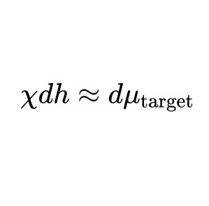
Given a target change $d\mu_{\text{target}}$, we want the minimum-norm sample reweighting $dh$ such that $\chi\, dh \approx d\mu_{\text{target}}$. The solution is:

$$dh_{\text{opt}} = \chi^\dagger d\mu_{\text{target}} = \chi^T (\chi \chi^T)^{-1} d\mu_{\text{target}}$$

In practice, we form the Gram matrix $G = \chi \chi^T$ and add ridge regularization $G_{\text{reg}} = G + \alpha I$ (the intent and interpretation of this regularization is discussed in ). We solve for $v = G_{\text{reg}}^{-1} d\mu_{\text{target}}$ and project back: $dh_{\text{opt}} = \chi^T v$. The per-sample scores $s_i = (\chi^T v)_i$ tell us how much to upweight ($s_i > 0$) or downweight ($s_i < 0$) each training sample.

From $dh$ to training weights. The patterning equation produces a vector $\delta h \in \mathbb{R}^n$ that can take arbitrary sign and magnitude. To convert it into valid per-sample training weights, we start from the natural data weights $h_0$ (the Bernoulli base distribution over input types, normalized to mean 1), add the perturbation, floor at a small $\varepsilon > 0$ to prevent zero or negative weights, and renormalize:

$$h = \frac{\max(h_0 + \alpha\, dh;\, \varepsilon)}{\mathrm{mean}\bigl(\max(h_0 + \alpha\, dh;\, \varepsilon)\bigr)}$$

The scalar $\alpha$ controls the overall perturbation scale. Renormalization to mean 1 ensures the effective learning rate is unchanged. Note that the flooring and renormalization modify the actual applied perturbation: the prediction $\delta\mu_{\mathrm{pred}} = \chi \cdot (h - h_0)$ is the effective change in observables, not the raw output of the pseudoinverse. For small $\alpha$ these coincide; for large $\alpha$ the floor clips extreme negative entries.

The additive clipping scheme above is not the only option. We find that other methods of converting $dh$ into valid weights work comparably well, including exponentiating the scores ($h_i \propto \exp(\alpha \cdot dh_i)$), which avoids the flooring issue entirely. In general, the patterning step is not particularly sensitive to this choice (at least in this toy model); most reasonable schemes produce similar results, though some tuning of the perturbation scale $\alpha$ is needed. For the ridge parameter, we find values around $10^{-3}$ to work well; the interpretation of this choice in terms of the mode structure of $\chi$ is discussed in Section 4.3.0.1.

Training on the reweighted data. The patterning step produces a set of weights $h$; we then train the model for multiple gradient steps on the reweighted loss $L(w; h) = \frac{1}{n}\sum_i h_i \ell_i(w)$ before re-estimating $\chi$. How many steps to take is a design choice that we return to in .

Choosing Bifurcations

Susceptibilities tell us when the model is most sensitive to intervention and what effect different data perturbations will have. The patterning equation tells us which data perturbations are necessary to achieve a target effect. Now we test whether we can use this to choose the outcome of a bifurcation.

Starting from a perfect 4-gon with a single ‘dead’ feature at the origin, there are four gaps the new feature can grow into. In the language of observables, placing f4 between f0 and f1 means targeting $\phi_{\text{dot}[0,4]} = \phi_{\text{cos}[1,4]} = 0.309$ (the interior angle of a regular pentagon), leaving the angles between $W_4$ and non-neighbors unconstrained.

4-gon → 5-gonepoch 0/500

Gap 1

...

Gap 0

...

Gap 2

...

Gap 3

...

In biological development, bifurcations are controlled by the concentrations of different morphogens. Here, the per-sample weights $h_i$ play the same role. They define a concentration field over data space that the model is exposed to during training, and the patterning equation tells us which field to apply.

We compute the reweighting only once at the bifurcation point and train forward with the modified distribution (we extend this to an iterative procedure in the next section). Across all four gaps, patterning places the new feature in the specified location. Precision is high, though it varies somewhat with sparsity: in some regimes the transitions are sharper and easier to control than others.

Analytically Solving the 4->5 Gon Bifurcation

At the 4-to-5-gon transition, the dead feature $W_4$ sits at the origin. The total loss near this point turns out to be purely quartic in $|W_4|$: the quadratic term vanishes exactly due to a cancellation between interference costs and self-reconstruction benefits. The Hessian at the origin is the zero matrix.

This has two consequences. First, any method that relies on at most second-order information (including adaptive stochastic optimizers like Adam and classical influence functions) gets no signal at this point, and will struggle even in the vicinity of this point: the loss gradients with respect to $W_4$ are zero, so there is nothing for the Hessian to invert. Second, the angular structure that determines which gap the feature grows into lives entirely in the per-sample losses, not the total loss. This is the structure that susceptibilities detect and that patterning exploits.

Analytical treatment of the 4-to-5-gon transition

At the transition point, the system sits at a critical point—a saddle in the loss landscape. Near this saddle, the loss has the form:

$$L(\ell) \approx L_0 + a\ell^2 + b\ell^4$$

where $\ell = |W_{\text{new}}|$ is the magnitude of the new feature. When $a < 0$, the saddle becomes unstable and the feature spontaneously grows—but the critical point doesn’t specify which branch. That choice depends on which valley the system descends into.

Four active features form a regular square at unit norm, with the dead feature parametrised in polar coordinates: $W_4 = r(\cos\theta, \sin\theta)$. By parameterising in this way, the total loss turns out to be remarkably clean:

$$H(r, \theta) = 1 + r^4$$

The quadratic term in $r$ vanishes exactly, for all angles $\theta$. This cancellation has a satisfying origin: the interference that a growing $W_4$ causes on the four existing features contributes $+r^2$ to the loss (summing over the four quadrants via the tight-frame property of the square), while the self-reconstruction benefit of having a nonzero $W_4$ contributes $-r^2$ (from $\ell_4 = (1-r^2)^2 + r^2$). These cancel perfectly, leaving only the quartic. The Hessian at the origin is the zero matrix.

The posterior at this point factorizes in a useful way: the angle $\theta$ is uniformly distributed and independent of $r$, while $r$ follows the quartic distribution $p(r) \propto r,e^{-\beta r^4}$. While the total loss is independent of $\theta$, the individual per-feature losses are not. Each feature’s loss fills exactly one quadrant of the angle:

$$\ell_0 = r^2\cos^2\theta \cdot \mathbf{1} { \cos \theta > 0}, \quad \ell_1 = r^2\sin^2 \theta \cdot \mathbf{1} { \sin \theta > 0}, \quad \ldots$$

Feature 0’s loss is largest when $W_4$ points toward $W_0$, because that is where the interference is worst. This angular structure — invisible in the total loss but present in each per-sample loss — is what allows data reweighting to steer the direction of growth.

Observable

$\phi_{\text{dot}[0,\,4]}$

$\phi_{\text{dot}[1,\,4]}$

$\phi_{\text{dot}[2,\,4]}$

$\phi_{\text{dot}[3,\,4]}$

-7.72e-4

1.44e-5

8.09e-4

-3.14e-5

-6.92e-5

3.94e-5

-8.41e-4

-5.63e-6

8.24e-4

1.23e-6

7.52e-4

1.65e-5

-8.29e-4

4.84e-5

2.44e-5

-3.37e-5

8.09e-4

3.99e-5

-8.53e-4

-5.57e-5

$h_0$

$h_1$

$h_2$

$h_3$

$h_4$

Per-sample weight $h_i$

$\phi_{\text{dot}[0,\,4]}$

$\phi_{\text{dot}[1,\,4]}$

$\phi_{\text{dot}[2,\,4]}$

$\phi_{\text{dot}[3,\,4]}$

$-\alpha$

$\mathbf{0}$

$+\alpha$

$\mathbf{0}$

$\mathbf{0}$

$\mathbf{0}$

$-\alpha$

$\mathbf{0}$

$+\alpha$

$\mathbf{0}$

$+\alpha$

$\mathbf{0}$

$-\alpha$

$\mathbf{0}$

$\mathbf{0}$

$\mathbf{0}$

$+\alpha$

$\mathbf{0}$

$-\alpha$

$\mathbf{0}$

$\phi_{\text{dot}[0,\,4]}$

$h_0$

$h_1$

$h_2$

$h_3$

$h_4$

Per-sample weight $h_i$

Computing the covariances under the quartic posterior gives the susceptibility of the dot product observables in closed form, depicted above. The susceptibilities tell us that increasing the weight on feature $i$‘s data pushes the dead feature away from feature $i$ and toward the diametrically opposite feature, because the added weight penalizes interference in that direction. Orthogonal features have zero effect on each other’s angular susceptibility. The dead feature’s own weight $h_4$ does not bias the angular direction at all — it is a uniform destabilizer, controlling whether the feature grows but not where.

The moments where developmental control matters most are precisely the singular points where classical methods fail. This is not a limitation of a particular implementation; it is a structural feature of bifurcations. The signal that patterning needs lives in higher-order geometry that the Hessian cannot see. Hence the need for more powerful techniques like patterning.

We can similarly pattern the 3 to 4 transition, targeting an angle of 60 degrees between the new feature and two neighbors.

3-gon → 4-gonepoch 0/500

Gap 0

...

Gap 1

...

Gap 2

...

Patterning

The patterning equation gives us a gradient in the space of data distributions. Sometimes a single step along this gradient tilts the loss landscape such that our targets are immediately obtainable. In the previous section, we applied a single patterning step to control a bifurcation – compute the reweighting once, train forward. This is enough when the path to the desired posterior is direct. However, the real power lies in iteratively following this gradient: estimate susceptibilities at the current weights, compute a new reweighting, train, and repeat. This carves a trajectory through data-space, much like how weight-space gradient descent is used to train models, and is patterning proper.

In Section 5.1, we describe this loop. In Section 5.2, we demonstrate it by swapping two features in a trained 5-gon, moving between two global minima separated by a large loss barrier. In Section 5.3, we step back and consider what patterning is doing geometrically: tracing a trajectory not through weight space but through the space of loss landscapes.

The Patterning Loop

The simplest version of this loop is as follows:

[Bilevel optimization: A series of panels showing contour plot of a loss landscape. We see a starting mode and a target mode (even though “modes” is a wrong concept it’s fine here) labeled on the first panel. From left to right, we see the loss landscape morphing slightly as the landscape goes through a second order phase transition that annihilates the two modes against each other in the middle and then pulls them apart again. Within each panel we see a small SgD run converge from the previous local minimum to the new modified local minimum. As we cross the annihilation, SGD ends up on the other side of the newly forming energy barrier, and we end up at the final target mode.]

Rewriting Minima

By controlling bifurcations we choose which valley Waddington’s marble descends into. But what about moving between valleys — taking a model that has already settled and pushing it somewhere else?

In Waddington’s original picture, this is forbidden. The ridges between valleys grow steeper as the marble descends; a differentiated cell cannot become a different cell type. For decades, biologists believed this was a one-way street. Then in 2006, Shinya Yamanaka showed that a handful of transcription factors could reprogram adult cells back into stem cells — the marble could be pushed back up the hill.

We take a trained 5-gon and ask: can we rearrange its features into a specified configuration? The target has the same loss as the original (by symmetry of the polygon), but there is no low-loss path between the two under the natural data distribution — each is a global minimum separated by a loss barrier.

Because patterning can reweight data samples, we don’t need to follow the gradient on the original loss — we can reshape the landscape itself. We change which data the model sees, and what was a ridge becomes a valley. The marble still rolls downhill, but downhill now leads somewhere new.

Classifying Targets

Our observables are the ten pairwise cosine similarities $\hat W_i \cdot \hat W_j$ and the five feature norms $\|W_i\|$. Because every target is a rearrangement of the same regular pentagon, all norms are identical across targets — the targets differ only in which features are adjacent and which are not.

On a regular pentagon, the cosine between two features takes one of just two values, determined by whether the features are adjacent (gap 1, one edge apart) or non-adjacent (gap 2, two edges apart) on the original ring. A target is therefore fully specified by its gap pattern: for each pair of positions on the ring, are the two features placed there gap-1 or gap-2 apart?

Many different-looking rearrangements produce the same gap pattern. For instance, the 3-cycle $(f_1\;f_2\;f_3)$ and the double swap $(f_1\;f_2)(f_3\;f_4)$ place different features at every position, yet at every position pair the gap between the features placed there is the same — so the two rearrangements define the same target. This happens because one arrangement can be obtained from the other by relabeling all features via a rotation of the pentagon, which preserves all gaps.

gap 1

gap 2

$\mathrm{id}$

All edges gap 1

$(f_1\;f_2\;f_3)$

$(f_1\;f_2)(f_3\;f_4)$

x

Working out which rearrangements are observationally distinct, we find exactly 12 gap patterns — the 120 permutations of five features, modulo the 10-element dihedral group $D_5$ of rotations and reflections. One is the identity. The remaining 11 non-trivial targets are naturally organized by how many of the five original neighbor pairs they destroy — the break count.

$\mathrm{id}$

$(f_3\;f_4)$

$(f_2\;f_3)$

$(f_2\;f_4)$

$(f_1\;f_2)$

$(f_1\;f_3)$

≡

≡

≡

≡

2-breaks. Two features the starting polygon exchange positions. The rest of the polygon is undisturbed — three of the five original neighbor pairs survive. Any single swap between features falls in this class, and all are equivalent under $D_5$. For example, swapping f2 ↔ f3 and swapping f4 ↔ f1 are the same task: both swap a pair of adjacent features, and the starting polygon’s rotational symmetry maps one to the other.

$(f_1\;f_3\;f_2)$

$(f_2\;f_4\;f_3)$

$(f_1\;f_2\;f_3)$

$(f_2\;f_3\;f_4)$

$(f_1\;f_2)(f_3\;f_4)$

≡

≡

≡

≡

3-breaks. Only two of the five original neighbor pairs survive. Each 3-break target can be described equally well as a 3-cycle rotating three features or as two simultaneous swaps — these very different operations produce the same gap pattern at every position pair, so they define the same observable target. All five 3-break targets are equivalent under $D_5$.

$(f_1\;f_3\;f_4\;f_2)$

The 5-break. Every neighbor relationship in the starting polygon is changed. There is exactly one such target (up to $D_5$): the features are maximally scrambled so that no original neighbor pair remains adjacent. Naturally, there is only one such permutation of this type.

A rearrangement can break 0, 2, 3, or 5 of the five original neighbor pairs. Break counts of 1 and 4 are impossible: four intact edges of the pentagon necessarily form a path whose two endpoints are adjacent, but the single remaining step would need to connect non-adjacent features — a contradiction. (By a duality that swaps gap-1 and gap-2 steps, the impossibility of 1-break implies the impossibility of 4-break.)

The dihedral symmetry of the starting pentagon makes all targets with the same break count equivalent patterning problems: a $D_5$ rotation or reflection maps any one to any other, so the susceptibility structure, data reweightings, and patterning trajectory are identical up to relabeling of features. Using this target-taxonomy, we are able to succinctly study all possible ways to pattern between pentagons. We do so in this next section.

Trajectories in the Space of Data Distributions

Over the course of patterning a trajectory is traced through the space of data distributions. This trajectory inherently has a dual — the trajectory of the model through parameter space. As the model’s internal structure evolves, its susceptibilities change, and so interpretable structure visible in susceptibilities is carried through to interpretable structure in the perturbations the patterning compiler is making to the data distribution.

What does this trajectory look like? We study our break classes, starting with the 2-break, swapping features 0 and 1. The heatmap below shows the per-input weights $h_i$ at each patterning step.

Loading...

Each row is an input type (labelled by which features are active); each column is a step; color indicates the weight.

3-break5-break

Loading...

The figure above shows this trajectory for the feature swap. Each row of the heatmap is an input type (labelled by which features are active); each column is a patterning step; color indicates the accumulated sample weight $h_i^{(t)}$.

Two things are immediately visible. Firstly, we can clearly see several phases consisting of different inputs being upweighted. Early on while still approaching the crossover (which happens at epoch 97) the weights are in fluctuation — work is being done to bring features zero and one together. Once feature zero is on the right hand side of feature one (the features have crossed), the work is mostly done — the natural, unweighted structure of the loss landscape would be enough to reach the target. After the successful crossover the weights stabilize until the permuted 5-gon is reached.

Secondly, weightings are interpretable.

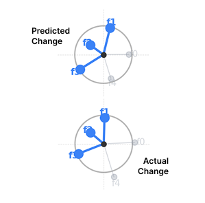
Let’s examine what $\chi$ ‘thinks’ its data weights are going to do to the model. We can check this by, as before.

Both the upweighted ($>1\times$) and downweighted ($<1\times$) inputs are easy to understand. On the upweighting front, input (1,0,0,0,1) pushes $f_0$ and $f_4$ apart. In doing so $f_0$ moves inward towards $f_1$ (nice!) and $f_4$ towards $f_3$; input (0,1,1,0,0) does a symmetric thing, pushing $f_1$ and $f_2$ apart, similarly moving f1 and f0 together; input (1,0,1,0,0) drags $f_0$ and $f_2$ upwards – finally, input (0,1,0,0,1) is it’s symmetric partner, driving f1 up and across. At epoch 7 these four inputs are nearly the only inputs being upweighted – linearly combining their movements.

Loading...

Each column of $\chi$ shows a single input’s predicted effect on all 15 observables. The patterning equation produces a linear combination of these observable changes: find per-input weights such that the weighted sum of all these per-input effects adds up to the desired structural change.

The Patterning Controller

The idea that statistical observations of a system’s behaviour can provide the information needed to control it — without requiring a mechanistic model of its internals — is among the founding insights of modern control theory (Wiener, 1948). The framework is general: a plant is the system being steered, a controller observes its output, compares it to a target, and computes an intervention. The gap between target and output is the tracking error. The loop closes when the intervention changes the output, which changes the tracking error, which changes the next intervention.

The patterning loop wraps the susceptibility computation in a feedback controller. At each step, the controller observes the current structure (measuring observables $\mu_t$), estimates the plant (computing $\chi_t$), computes an intervention (solving for $dh_t$), applies it (training on the reweighted loss), and repeats.

The loop as written re-estimates \chi on a fixed schedule. We can do better by doing so only when needed. Between recomputations, the model follows the gradient of the reweighted loss; as long as the landscape is still guiding it toward the target, we are still the current estimate of \chi has nothing to add. It is only when training plateaus — when the current weights have done all they can — that re-estimating is worth the cost. This is event-triggered control (astrom_event_triggered): sample the plant when the output stalls, not on a clock.

However, we do not have $\chi$ as a given property of the system; we estimate it from finite posterior samples at every step. This is the setting of adaptive control, and the specific construction patterning implements is the self-tuning regulator (Åström & Wittenmark, 1973): estimate the plant from data, compute the optimal action as if the estimate were exact, apply it, re-estimate, repeat. The assumption that the current estimate is correct when computing the action is called certainty equivalence. It is a working hypothesis rather than a theorem, and its reliability depends on how much of $\chi$ is actually resolved by our sampling.

Rather than estimating the plant on a fixed schedule, we can let the system tell us when it needs new instructions. Between recomputation points, the model trains on fixed sample weights, following the gradient of the reweighted loss. As long as the model is not at a minimum of this loss the model will keep changing. However, when training plateaus the juice has run out. The current weights have done all they can, and we need to re-estimate χ and compute a fresh perturbation.

The resulting controller is remarkably efficient. We test one representative target from each class, comparing three patterning regimes: single-step (one data reweighting, then train to convergence), periodic recomputation (re-estimate $\chi$ every 10 epochs), and adaptive recomputation (re-estimate when the weighted loss plateaus).

When patterning on a 3-break target, a fixed schedule of one susceptibility estimate every 10 epochs takes about 120 epochs to reach the correct permutation, and around 230 to settle into a perfect 5-gon: this is 12 and 23 patterning steps, respectively. By sparsely computing susceptibilities, as few as 3 patterning steps to reach the correct permutation and a single extra to hit the perfect 5-gon. This works because the recompute, when properly calibrated, fires precisely at structural boundaries: when features begin to move, when they cross, and when they need to settle into their new positions.

TODO: Talk about minimal weight interventions and phases

Mode Structure in the Plant

Multivariable control concerns itself with systems of multiple inputs and outputs. In multivariable control the central object is the plant’s gain matrix. Its singular value decomposition decomposes the input–output relationship into independent control channels ranked by effectiveness. The singular values are called the principal gains: the largest tells you the direction in which the system is most responsive, the smallest tells you the direction in which it is hardest to steer (Skogestad & Postlethwaite, 2005). Our $\chi$ plays the role of the plant, with data reweightings as control inputs and structural coordinates as outputs.

Writing $\chi = \sum_j \sigma_j, u_j v_j^T$, each mode $j$ pairs a direction $u_j$ in observable space with a direction $v_j$ in data space. The singular value $\sigma_j$ is the gain of that channel, and it tells us how strongly a unit perturbation along $v_j$ moves the model along $u_j$. Leading modes are easier to steer, later modes are harder.

In our setting, where we estimate $\chi$ via sampling, singular values of $\chi$ also tell us about how well estimated a response is. So the mode ranking carries a double meaning, where leading modes are not only the most effective control channels but also the most reliably estimated. Trailing modes are simultaneously the weakest levers and the least trustworthy ones. The condition number $\sigma_1/\sigma_k$ sets the practical limit on how many independent structural directions patterning can steer at once.

This gives a natural interpretation to the role of the ridge regularization we use (discussed ). Rescaling $1/\sigma_j \to \sigma_j/(\sigma_j^2 + \alpha)$ preserves the ordinary inverse response on large modes and suppresses it on small ones.

Related Work

This work sits at the intersection of several research areas: singular learning theory, data attribution and optimization, constrained optimization, and alignment. We survey each below, organized around how patterning relates to and differs from existing approaches.

Singular Learning Theory and Developmental Interpretability

Patterning comes most directly out of a research agenda we have been developing over the past three years [devinterp2023, metaunialign2023], applying singular learning theory (SLT; Watanabe (2009)) to interpretability and alignment.

What is singular learning theory? First, some background: many classical results in learning theory (including asymptotic normality, the Bayesian Information Criterion, the Bernstein–von Mises theorem) assume regular models, that is, models whose loss landscapes have isolated, locally quadratic minima. For neural networks, this assumption fails. The loss landscape is degenerate, with non-isolated minima with Hessians that have zero eigenvalues. The classical results that were built on regularity do not apply.

Singular learning theory relaxes the regularity assumption and generalizes many of the classical results to the singular setting. It is a theory of Bayesian learning, for which the learning process is governed by Bayes’ rule as the dataset size $n$ grows, rather than by gradient descent dynamics in increasing timestep $t$. Watanabe’s central result (Watanabe 2009) derives closed-form asymptotics for (in-distribution) generalization error in the large-data limit, replacing the parameter count in the BIC with a geometric invariant known as the real log canonical threshold (RLCT) or, alternatively, the learning coefficient.

The developmental interpretability agenda. The developmental interpretability agenda (devinterp2023) began with several key hypotheses. First, that Watanabe’s Bayesian theory could serve as a productive idealized model of SGD-based training. This has borne out empirically across a series of works spanning toy models and now increasingly larger language models (todo). Second, that SLT could be extended beyond the asymptotic, in-distribution, Bayesian setting into a more general theory of deep learning, even at finite dataset sizes and in other limiting regimes, even under distribution shifts, and even for non-Bayesian learning algorithms.

Susceptibilities [lang2, lang2_5, lang3, sf1, sf2, sf3] are the first step towards the second extension: they measure the first-order correction to posterior expectations under a vanishing shift in the data distribution, and form the basis of our approach to interpretability, which we call “Spectroscopy”. This provides a principled route towards understanding how model internals and behaviors respond to changes in the data distribution.

Patterning, introduced by wang2026 and applied to the TMS here, provides evidence for the last extension. The results in Section TODO demonstrate that predictions derived from the Bayesian posterior successfully predict how SGD training responds to perturbations of the data distribution. This was not guaranteed by the theory. It is an empirical finding that supports the eventual unification of Bayesian and optimization-based perspectives on deep learning.

Influence Functions and Data Attribution

Susceptibilities are a generalization of influence functions. Influence functions [cook1982, koh2017] measure the sensitivity of model predictions to changes in training data importance. This can be seen as a special case of a susceptibility where the perturbation is a per-sample weight (the same as considered here) and the posterior can be approximated as Gaussian (kreer2026):

$$\chi_{k,i}^{\text{IF}} = -\nabla\phi_k^T H^{-1} \nabla\ell_i,$$

where $H=\nabla^2 L_n(w)$ is the Hessian at the local minimum.

Influence functions face two major problems, one practical and one theoretical. The practical problem is that Hessian inversion is intractable for large models. The theoretical problem is the Hessian inverse is not even well-defined for neural networks. Susceptibilities solve both.

Susceptibilities bypass the Hessian inversion. Many methods within the field of training data attribution (TDA) can be understood as approximations to the full Hessian inverse. This includes EK-FAC (grosse2023), TRAK (park2023), DataInf (kwon2024), and even the simple inner product of gradients.

Estimating susceptibilities bypasses the Hessian inversion step entirely by directly computing statistics over the local loss landscape. This comes with a different set of scaling exponents that in many cases outperforms Hessian-based methods (alexander2026).

Susceptibilities measure influence at all orders. Classical influence functions assume that the model is at an isolated local minimum with an invertible Hessian $H$. These are precisely the same regularity assumptions we discussed previously that break down for neural networks. As a consequence of this breakdown, the empirical Hessian inverse is technically ill-defined. This can be “fixed” by regularizing the Hessian, $H \to H + \lambda \mathbb 1$, but, as we saw in Section TODO, this is not enough: at the 4-to-5-gon bifurcation, the Hessian is exactly zero and contains no information about which branch the model will take. Regularizing $H$ makes the matrix invertible but does not conjure any new signal.

Understanding the response of the model in general, especially at bifurcations, requires going to fourth order in loss landscape geometry. This is exactly the information that is available to susceptibilities.

Data Optimization

The idea of optimizing the data distribution to shape what models learn has a long history.

Data optimization as bilevel optimization. The most general framing is bilevel optimization over data weights [ren2018, shu2019]: minimize an outer objective $L$ defined in terms of a model trained on a weighted dataset:

\boldsymbol{h} = \underset{\boldsymbol h}\text{argmin} L(w^*(\boldsymbol h)).

By applying the chain rule and invoking the implicit function theorem, the hypergradient for sample $i$ is precisely the classical influence function

$$\grad_{h_i} L = -\nabla L^\top H^{-1} \nabla \ell_i.$$

Data optimization in practice. Actually implementing this is highly intractable, even with state-of-the-art influence function approximations, because the influence functions have to be calculated repeatedly over the course of training. Therefore, in practice, the use of influence functions is reserved to one-time interventions and ad-hoc rules (e.g., filtering to remove samples below a certain threshold, or implementing a heuristic schedule based on influence rankings, see, e.g., iffair2025, li2025, self_influence2023).

In fact, most work abandons influence functions altogether, relying instead on heuristic proxies rather than actual response signals. The current state-of-the-art in actual practice optimizes at the level of domain mixture weights rather than individual samples (e.g., DoReMi, DoGE, RegMix, and related methods). This trains proxy models to predict loss contributions or extrapolates from granular mixture-level scaling laws.

There are several closely related problems to data mixture optimization. For example, curriculum learning focuses on ordering samples rather than weighting samples. Here, it is common to order samples by an increasing measure of difficulty [bengio2009, kumar2010, graves2017]. Meanwhile, data pruning and coreset selection [sorscher2022, toneva2019] restricts reweightings to binary include/exclude decisions.

How patterning generalizes this. The preceding section established that susceptibilities generalize influence functions as a response signal. Patterning can be understood as enforcing two changes on the bilevel optimization framing. First, we replace the point estimate of the outer objective with an expectation value. Second, we replace the scalar target with a specification of multiple objectives. How the resulting reweighting is applied (additive update, mirror descent on the simplex, or other) is a separate design choice downstream of both frameworks.

Constrained Optimization

Training against multi-objective specifications rather than loss alone connects patterning to a broader literature on constrained learning. The key distinction is between what is being optimized (parameters vs. data distribution) and where the constraints are imposed on (behavioral outputs vs. internal structure via expectation values).

Penalty methods are the simplest approach. These add weighted regularization terms to the loss for each additional target. This approach is limited however (ramirez2025), because there need not be penalty coefficients that simultaneously satisfy all constraints and tuning the relative coefficients introduces costly hyperparameter tuning overhead.

Lagrangian and primal-dual methods (chamon2020; chamon2021; cotter2019; gallego2022) address this limitation by making the penalty coefficients themselves learnable. The dual variables $\lambda_i$​ adapt during training: when a constraint is violated, its multiplier increases; when it is satisfied, the multiplier decreases or vanishes. Constrained Policy Optimization (achiam2017) and its successors enforce similar cost constraints in an RL setting throughout training via trust-region or primal-dual updates over policy parameters.

Patterning shares the core insight that training should be formulated against specifications, and its iterative loop — re-estimate susceptibilities, compute target-driven weights, train, repeat — has the same feedback-control structure as primal-dual optimization: the per-sample weights $h_i$​ in patterning play an analogous role to the dual variables $\lambda_i$​ in Lagrangian methods, both adapting iteratively to drive the system toward a specification. But patterning differs in what is being optimized and where the specification lives. Constrained learning methods optimize over model parameters, subject to constraints on model outputs (e.g., fairness rates, robustness margins, worst-case loss on subpopulations). Patterning optimizes over the data distribution, targeting internal structure via expectation values of observables under the local posterior. The constraints are on the geometry of the loss landscape and thus internal structure, not on predictions. And because the specification is expressed in terms of posterior expectations rather than point-valued constraint functions, patterning remains well-defined at the singular points — bifurcations, phase transitions — where the constraint gradients that Lagrangian methods rely on degenerate.

Alignment

All current alignment techniques are effectively soft forms of constrained data optimization.

Alignment is data optimization. We use the same basic deep learning techniques but with empirically and heuristically chosen datasets. SFT is just finetuning on curated examples; RLHF is RLVR with binary feedback signal coming from a learned reward model that has distilled an implicit alignment specification; DPO collapses this into a direct loss on preference pairs; Constitutional AI and deliberative alignment generate training data conditioned on a specification of natural language principles. The alignment signal in each case lives in the data.

The design of these curricula is driven largely by evolutionary search. Labs try different mixtures, train different models, and iterate on what works best. This may very well work. Or we may need to substitute in a more principled way to learn data curricula. Traditional bilevel optimization using IFs is both intractable and underpowered. Patterning with susceptibilities offers a route to addressing both.

Alignment is constrained optimization. What these methods share is an indirect relationship between the alignment specification and the resulting model structure. In RLHF, the specification is implicit in the preference data — whatever patterns annotators happen to reward, compressed into a scalar signal by the reward model. In Constitutional AI, the specification is more explicit (natural language principles) but the translation to training signal passes through an opaque chain of AI critique, revised responses, and preference labels. In all cases, the practitioner specifies desired behavior through examples and hopes the model develops the right internal structure to generalize that behavior correctly.

Patterning offers a more direct path. Instead of specifying alignment through examples of preferred outputs, it specifies alignment through structural observables — expectation values that characterize the model’s internal geometry. Susceptibilities provide a differentiable mapping from “what structural change do I want” to “what data change produces it.” The claim is not that patterning replaces RLHF or DPO. It operates at a different level: current methods specify what outputs should look like; patterning can specify what internal structure should look like. These are complementary.

The open question is the compilation step: translating alignment desiderata (“be honest,” “don’t pursue power”) into constraints on expectation values. For the toy model, this is trivial. For real models, this is the hard part, and it is the same hard part that interpretability faces. Susceptibility-based interpretability [baker2026, gordon2026] provides a starting point by discovering observables from the posterior itself. The vision is a closed loop: interpretability discovers the structural vocabulary, patterning targets it, and the result is alignment that operates on internal structure rather than surface behavior.

Discussion

In this section, we step back from the specific results and consider what they mean for the broader project of understanding and controlling neural network development.

From Reading to Writing

The conceptual arc of this post mirrors a progression in biology: from anatomy (describing structure) to developmental biology (understanding how structure forms) to synthetic biology (controlling what structure forms). In the language of neural networks, this is the progression from mechanistic interpretability to developmental interpretability to patterning — and from models that are grown to models that are crafted.

The theoretical foundation for this progression is Structural Bayesianism (troiani2025): the hypothesis that the geometry of the loss landscape faithfully reflects a model’s internal computational structure. If this is right, then posterior expectation values provide a coordinate system over the space of possible internal structures. Optimizing these coordinates is optimizing structure itself; this is the natural way to do interpretability-guided training.

Patterning makes this actionable. Over the course of a patterning run, the per-sample weights trace a trajectory through the space of data distributions. But a data distribution is more than a list of weights. It defines a loss landscape $L(W; h) = \sum_i h_i \ell_i(W)$, and therefore a posterior, each with its own critical points, basins, and bifurcation structure. A trajectory through data space is a trajectory through the space of loss landscapes.

If we had complete access to this space, we could ask structural questions directly. Which internal configurations exist as stable minima under some data distribution? Given two configurations, is there a continuous path through data space along which one minimum deforms into the other without crossing a barrier? Where are the catastrophe surfaces — the data weightings at which the qualitative structure of the landscape changes, where minima appear, merge, or vanish?

These questions are intractable to answer exhaustively, even for our 10-parameter model. What patterning provides is a tractable way to search through this space, guided by local measurements of its geometry. The feature swap in Section TODO demonstrates that this search can find paths between configurations separated by loss barriers — paths that exist in data space even when no gradient path connects them in weight space.

Why Singularities Are Where Control Lives

A recurring theme in this work is that the moments where control matters most are precisely the moments where standard methods fail. The 4-to-5-gon bifurcation is the clearest illustration. At the bifurcation point, the Hessian is exactly zero. Any method that approximates the loss landscape as locally quadratic — including influence functions, natural gradient methods, and second-order optimizers — gets no signal. The bifurcation is invisible to them.

The posterior, by contrast, captures the full geometry: the quartic potential, the angular structure of per-sample losses, and the resulting susceptibilities that encode the branching structure of the bifurcation. The anomalous $\beta$-scaling of the susceptibilities ($\beta^{1/4}$ and $\beta^{1/2}$ rather than the regular $\beta^1$) is the fingerprint of this singularity — a direct measurement of higher-order geometry that no Gaussian approximation can reproduce.

This is not a peculiarity of toy models. Neural network loss landscapes are generically singular: weight-space symmetries, parameter redundancies, and phase transitions all produce degenerate critical points where the Hessian fails to capture the relevant geometry. Much of the machine learning literature implicitly assumes regularity — that the Hessian at a trained model tells you what you need to know about the local landscape. For neural networks, this assumption breaks down at the points that matter most: the bifurcations, phase transitions, and symmetry-breaking moments where the model is deciding what internal structure to develop.

A common objection runs: “I accept that symmetries reduce the effective dimensionality. But you’re claiming the geometry involves terms like $x^4$ and $x^6$. Why should I believe higher-order structure matters?” The burden of proof runs in the opposite direction. Regularity — the assumption that the geometry is entirely captured by the Hessian — is a very strong condition that holds only for a measure-zero set of models. The question is not “why should singularities matter?” but “why would you assume they don’t?” The bifurcation analysis in this post provides what is, to our knowledge, the strongest concrete demonstration of the practical consequences: a setting where the qualitative outcome of training depends entirely on geometry that is invisible to second-order methods.

This is the domain of singular learning theory. The tools we have used throughout — the local posterior, expectation values, the local learning coefficient, susceptibilities — are all SLT constructions. They were designed for exactly this situation: characterizing and exploiting the geometry of singular loss landscapes. The results of this post suggest that the same tools can be used not only to read that geometry (spectroscopy) but to write it (patterning).

Limitations and Open Problems

Why Not Just Train Against the Observables?

In this toy model, one could achieve the same level of structural control via standard constrained optimization techniques like adding penalty terms for our dot product observables. At the bifurcation, this would break the rotational symmetry and pick out a unique direction. Why then invoke the machinery of susceptibilities and patterning?

This objection is valid for the TMS setting in particular, but not in general. The model’s structure is simple enough that structural observables can be written as differentiable functions of the weights. In this case, constrained optimization would work. The objection fails in general for two reasons.

First, expectation values carry information that point estimates do not. It may not always be the case that simple observables can be written down which isolate the structural information at a point value. wang2026 demonstrates that patterning can choose between two minima with identical loss, that are distinguishable only by their local geometry. This case requires more powerful control over expectations.

Second, in practice, the primary way we modify the training objective is already by modifying the data. As discussed in Section TODO, when we lack explicit structural observables (which is the generic case for real models), “optimizing against the target” means reweighting data, and doing so in a principled way is exactly what the patterning equation provides.

How to Choose Observables?

In the toy model of superposition, an appropriate set of structural observables are easy to identify: dot products and norms fully characterize the polygon geometry. Real neural networks do not come with such a convenient reparameterization. Discovering the appropriate set of structural observables for a given model is an open problem, perhaps the main difficult problem; this is what interpretability is about.

Prior work on susceptibility-based interpretability [baker2026, wang2025, gordon2026] suggests a path forward: begin with a broad (highly redundant) set of observables (per-sample losses, per-component losses, activation statistics, etc.), compute susceptibilities, and use the mode decomposition to discover which combinations of observables and data perturbations couple most strongly. This analysis itself guides the search toward more informative observables, for instance, by telling us how to explicitly target the low-gain modes to resolve them further.

There is a hard constraint here. The patterning equation can only achieve target changes that lie in the column space of the susceptibility matrix $\chi$. Any component of the target in the null space of $\chi^T$ is unreachable by data reweighting alone. This means the observable set must be expressive enough to span the structural directions you care about. Expanding this coverage requires more observables and more compute (additional forward passes per SGLD draw), creating a direct tradeoff between control resolution and computational cost.

Can We Resolve the Relevant Observables?

The SVD decomposition of $\chi$ reveals that the directions easiest to estimate are also the directions easiest to control, and vice versa, see section TODO. Leading modes have high gain and high signal-to-noise; trailing modes have low gain and are potentially indistinguishable from sampling noise.

This poses a problem for alignment. If the structural features most relevant to safety (honesty, corrigibility, etc.) live in the low-gain tail of $\chi$‘s spectrum, then patterning lacks leverage precisely where it matters most. We expect that patterning may enable an essentially complete solution to the Sharp Left Turn (soares2022) in principle, by giving us direct control over which structures form and how they generalize. But that control is only as good as our measurements. If the susceptibility spectrum cannot resolve alignment-relevant structure, we have traded an inductive bias problem in the model for a resolution problem in the measuring apparatus, and the outcome is the same.

There are reasons to be cautiously optimistic. Behavioral patterns that manifest broadly across the data distribution will couple to many samples and therefore appear as high-gain modes. The most consequential alignment-relevant patterns, such as power-seeking, are plausibly of this kind. More fundamentally, susceptibilities measure how the posterior would respond to a perturbation, not whether that perturbation has been observed. We expect that a catastrophic behavior does not have to be exhibited for its structural tendency to be detectable. We are actively investigating connections with elicitation (irving2025), where the goal is to find data perturbations that surface rare but dangerous behaviors. Whether patterning’s resolution extends to the full alignment-relevant spectrum remains open.

How Will it Scale?

The computational cost of patterning is dominated by SGLD sampling, which requires many forward passes to estimate posterior covariances. In the toy model, this is trivial. At scale, it is the primary bottleneck.

Our concurrent work on scaling spectroscopy demonstrates that susceptibility estimation is tractable for language models with over a billion parameters, using the same SGLD methodology. The patterning side — computing reweightings and training on modified distributions — has been demonstrated in small language models (wang2026) but not yet at the scale where it would be relevant for frontier alignment. Further engineering challenges include adapting to mini-batch training (where you cannot evaluate all samples simultaneously), handling the gap between population and empirical risk, and extending to reinforcement learning settings where the “data distribution” is generated by the policy itself.

Outlook

The results in this post demonstrate patterning in a setting where internal structure is immediately visible and the right observables are known in advance. The path to impact requires relaxing both of these conditions.

The most immediate next step is reward models. Current alignment pipelines depend critically on reward models that are known to develop simple, biased proxies for human preferences — the “love of lists,” sycophancy, and related phenomena documented in the reward model literature. These biases are plausibly instances of the same structural dynamics visible in TMS: at decision points in the reward model’s development, the model commits to simple proxy features rather than more complex but accurate representations of human values. If susceptibilities can identify these decision points and patterning can bias them toward the more complex branch, the result would be reward models that better represent what humans actually want. We are actively pursuing this direction.

More broadly, patterning suggests a different framing for what alignment could look like. Current methods specify desired behavior through examples and hope the model develops the right internal structure to generalize correctly. Patterning inverts this: specify the desired internal structure and compute the data distribution that produces it. The missing piece is the compiler — the map from alignment desiderata to structural observables. Building this compiler is the central open problem, and it is where interpretability and alignment meet. Susceptibility-based interpretability discovers the structural vocabulary; patterning targets it; the result is a closed loop from specification to structure.

We note that the ability to precisely control what models learn is inherently dual-use. The same techniques that could enforce alignment constraints could be used to train models toward undesirable structure — inserting backdoors, amplifying biases, or shaping models to pursue goals that are not aligned with their operators’ intentions. This is a general property of any increase in training methodology capability, not specific to patterning, but it is worth stating clearly given the precision of control demonstrated here.

Appendix

Additional Hyperparameters

TODO: Table with $I_i$ and other TMS parameters

Patterning as Policy Gradient

For readers familiar with reinforcement learning, a perhaps natural interpretation of patterning is that patterning is policy gradient on data distributions.

Consider the expected value of an observable under the posterior:

$$\mu(\lambda) = \mathbb{E}*{w \sim p(\cdot|D*\lambda)}[\phi(w)]$$

where $\lambda$ parameterizes the data distribution (e.g., sample weights). We want to find $\frac{\partial \mu}{\partial \lambda}$ to know how shifting the data affects the observable.

Using the REINFORCE trick, à la Williams, 1992:

$$\frac{\partial \mu}{\partial \lambda} = \mathbb{E}*w\left[\phi(w) \cdot \frac{\partial}{\partial \lambda} \log p(w|D*\lambda)\right]$$

The posterior is $p(w|D_\lambda) \propto \exp{-\beta L_n(w|D_\lambda)} \varphi(w)$, so:

$$\log p(w|D*\lambda) = -\beta L_n(w|D*\lambda) + \log \varphi(w) - \log Z(\lambda)$$

Taking the derivative:

$$\frac{\partial}{\partial \lambda} \log p(w|D_\lambda) = -\beta \frac{\partial L_n}{\partial \lambda} - \frac{\partial}{\partial \lambda}\log Z(\lambda)$$

The partition function term is a baseline:

$$\frac{\partial}{\partial \lambda} \log Z = \frac{1}{Z} \int e^{-\beta L_n} (-\beta) \frac{\partial L}{\partial \lambda} \varphi , dw = -\beta \mathbb{E}\left[\frac{\partial L}{\partial \lambda}\right]$$

Substituting back:

$$\frac{\partial}{\partial \lambda} \log p(w|D_\lambda) = -\beta\left(\frac{\partial L}{\partial \lambda} - \mathbb{E}\left[\frac{\partial L}{\partial \lambda}\right]\right)$$

Therefore:

$$\frac{\partial \mu}{\partial \lambda} = -\beta , \text{Cov}\left(\phi(w), \frac{\partial L}{\partial \lambda}\right)$$

This is exactly the susceptibility formula. In RL terms:

• Policy: the data distribution $p(x|\lambda)$
• Environment: training dynamics that map data → trained model
• Reward: the observable $\phi(w)$ we want to maximize
• Policy gradient: $\frac{\partial \mu}{\partial \lambda}$ tells us how to adjust the data distribution

The key difference from standard RL: we don’t need to sample trajectories. The posterior $p(w|D_\lambda)$ (estimated via SGLD) gives us the entire distribution over “outcomes” (trained models) for a given “policy” (data distribution). We can compute the policy gradient analytically as a covariance.

@misc{adam2026patterning,
  title={Patterning Toy Models of Superposition},
  author={Max Adam and Jesse Hoogland and Daniel Murfet},
  year={2026},
  howpublished={\url{https://timaeus.co/research/2026-04-24-patterning-tms}},
  url={https://timaeus.co/research/2026-04-24-patterning-tms}
}