From Influence Functions to Statistical Physics

We recently published a series of papers that establish the Bayesian Influence Function (BIF) (Kreer et al. 2025; Adam et al. 2025; Lee et al. 2025). In this post, we introduce the BIF as a natural generalization of classical influence function methods. We show that the BIF resolves some conceptual and computational problems with classical TDA, and connect the BIF to susceptibilities, loss landscape geometry, and training dynamics. This provides justification for the developmental interpretability agenda and leads us to argue for a stagewise approach to data attribution.

Theory of Influence

Training data attribution (TDA) is usually framed as a leave-one-out question: how would sample $j$‘s loss change if sample $i$ were removed from training? For modern neural networks, that framing is both computationally expensive and conceptually unstable, because training is stochastic. We argue for a different starting point by defining influence as the response of the expected loss under sample reweighting. This leads naturally to the Bayesian influence function (Kreer et al. 2025).

What Is Influence?

The basic question of training data attribution (TDA) is: what effect does sample $i$ have on the model’s behavior on sample $j$? This is usually operationalized in terms of how the loss $\ell_j(w)$ changes when you train with or without sample $i$.

$$\ell_j(w^*(D)) - \ell_j(w^*(D^{\setminus i})),$$

where $D$ is the dataset, and $w^*$ is the trained set of weights.

Unfortunately, this leave-one-out formulation faces practical and conceptual problems in the modern deep learning paradigm.

Practically, the cost of training large deep neural networks makes it prohibitive to retrain models for many different datasets. Conceptually, the formula doesn’t even make sense: initialization, batch learning schedules, and GPU numerics conspire to make the training process fundamentally stochastic. Sample $i$ has no unique effect on the model’s behavior on sample $j$. It has a distribution of effects.

The easiest way to resolve the conceptual issue is to instead study quantities like the change in expected loss,

$$\mathbb{E}[\ell_j(w)](D) - \mathbb{E}[\ell_j(w)](D^{\setminus i}),$$

where $\mathbb{E}$ is an expectation over relevant sources of training stochasticity.¹ Of course, this makes the practical problem many times worse, because estimating even just a single expectation value requires many independent training runs. But we are making progress.

As a final trick, let’s generalize the question further. Instead of asking what effect does including/excluding sample $i$ have on my training process, ask: how does sample $j$‘s behavior change as we continuously vary the number of copies of sample $i$?

We rewrite our loss function as a weighted sum:

$$L(w)=\frac{1}{n}\sum_{i = 1}^{n}\ell_i(w) \to L^{\boldsymbol{\beta}}(w)=\frac{1}{n}\sum_{i = 1}^{n}\beta_i\ell_i(w),$$

where $n=|D|$ is the number of samples and $\beta_i$ is the importance weight of sample $i$. When $\beta_i=1$ we recover the original loss function. When we set $\beta_i=0$ we recover the loss on $D^{\setminus j}$. Now, we can continuously vary between these extremes and beyond.

Abusing notation, the final quantity we end up being interested in computing is:

$$\mathbb{E}[\ell_j(w)](\beta_i) - \mathbb{E}[\ell_j(w)](0)$$

Simplified further, because the second term can be recovered from the first, our problem has been reduced to the question of determining the function $\mathbb{E}[\ell_j(w)](\beta_i)$.

---

The Influence Expansion

We have a function $\mathbb{E}[\ell_j(w)](\beta_i)$ and we want to know how it depends on $\beta_i$. A natural approach is to use a Taylor expansion.

We start by fixing some reference choice of importance weights (or, equivalently, training dataset). For convenience, choose $\beta_i=1$, i.e., the “unperturbed” dataset that contains all of the query samples of interest. Write $\delta_i := \beta_i - 1$ for the perturbation away from this baseline, so that $\delta_i = 0$ is no change and $\delta_i = -1$ is leave-one-out. Then, we can obtain the “influence expansion”:

$$\mathbb{E}[\ell_j(w)](\delta_i) = \mathbb{E}[\ell_j(w)]\big|_{\delta_i=0} + \frac{\partial\,\mathbb{E}[\ell_j]}{\partial \delta_i}\bigg|_{\delta_i=0}\!\delta_i + \frac{1}{2}\frac{\partial^2\mathbb{E}[\ell_j]}{\partial \delta_i^2}\bigg|_{\delta_i=0}\!\delta_i^2 + \cdots$$

This is nice and general, but as stated, this has bought us no practical advantage yet. That requires a way to evaluate these derivatives cheaply. Then, we will have turned a hard problem (characterizing $\mathbb{E}[\ell_j(w)](\beta_i)$) into an infinite series of easy problems. If we’re lucky, we can get by just computing the first few terms and call it done.

Here, we’ll follow the developmental interpretability playbook[^devinterp] and replace the expectation over SGD trajectories with an expectation over the Gibbs measure

$$p_{\boldsymbol\beta}(w\mid D)= \frac{e^{-L^{\boldsymbol\beta}(w)}\varphi(w)}{Z(\boldsymbol\beta)},$$

where $\varphi(w)$ is a prior. In the case where $L^{\boldsymbol\beta}$ is a negative log likelihood, this is just the (tempered) Bayesian posterior. This replacement can be justified to some extent by the observation that, for many quantities of interest, late-stage SGD dynamics and the Bayesian posterior yield similar statistics (Mandt et al. 2017). But it is ultimately a modeling substitution that sacrifices some accuracy. Exactly characterizing the differences between the two learning problems remains a major open area.

Under this substitution, we can import the “derivative trick” from statistical physics, which lets us replace the derivatives in the influence expansion with cumulants over the unperturbed posterior. The central identity is:

$$\frac{\partial\,\mathbb{E}[\ell_j]}{\partial \delta_i} = -\text{Cov}(\ell_i(w),\, \ell_j(w)).$$

That is, the first-order influence of sample $i$ on sample $j$ is the negative covariance of their losses under the posterior. Repeated differentiation produces higher cumulants: the second derivative gives the third cumulant $\kappa_3(\ell_i, \ell_j, \ell_k)$, and in general the $r$-th derivative is $(-1)^r$ times the $(r\!+\!1)$-point connected correlation function. Crucially, all of these can be estimated from samples of the posterior — we no longer need to retrain for each perturbation.

The derivative trick

The derivative trick follows from differentiating the partition function. Recall that the Gibbs measure takes the form

$$p_{\boldsymbol{\beta}}(w \mid D) = \frac{1}{Z(\boldsymbol{\beta})} \exp\!\left(-\sum_i \beta_i \ell_i(w)\right) \varphi(w),$$

where $Z(\boldsymbol{\beta}) = \int \exp(-\sum_i \beta_i \ell_i(w)) \varphi(w)\, dw$ is the partition function. The expected loss on sample $j$ is

$$\mathbb{E}_{\boldsymbol{\beta}}[\ell_j(w)] = \int \ell_j(w)\, p_{\boldsymbol{\beta}}(w \mid D)\, dw.$$

Differentiating with respect to $\beta_i$:

$$\frac{\partial}{\partial \beta_i} \mathbb{E}_{\boldsymbol{\beta}}[\ell_j(w)] = -\mathbb{E}_{\boldsymbol{\beta}}[\ell_i(w)\, \ell_j(w)] + \mathbb{E}_{\boldsymbol{\beta}}[\ell_i(w)] \cdot \mathbb{E}_{\boldsymbol{\beta}}[\ell_j(w)] = -\text{Cov}_{\boldsymbol{\beta}}(\ell_i(w), \ell_j(w)).$$

The key step is that the derivative of the expectation brings down a factor of $-\ell_i(w)$ from the exponential, and the derivative of the normalization $Z(\boldsymbol{\beta})$ produces the product-of-expectations term that converts the raw second moment into a covariance. The same logic applies at each order: differentiating again with respect to $\beta_k$ yields the third cumulant, and so on. This is a standard identity in statistical mechanics, where differentiating the free energy $-\log Z$ with respect to external fields yields connected correlation functions.

Localizing Influence

The influence expansion is defined with respect to the global posterior over parameters compatible with the full dataset. That is the right formal starting point, but it is not usually the object we care about in practice. Influence is almost always queried relative to a particular checkpoint $w^*$: we want to know how losses respond over the distribution of training trajectories that interact with this model. Moving to a local posterior is also what makes the theory estimable, since it is exactly the form that can be sampled with scalable MCMC.

To do this, we replace the background measure $\varphi(w)$ with a localizer centered at $w^*$,

$$\varphi_\gamma(w\mid w^*) \propto \exp\!\left(-\frac{\gamma}{2}\|w-w^*\|^2\right),$$

where $\gamma$ controls the scale of locality. This induces a localized posterior

$$p_\gamma(w\mid D,\boldsymbol\beta,w^*) \propto e^{-L^{\boldsymbol\beta}(w)}\,\varphi_\gamma(w\mid w^*).$$

Large $\gamma$ restricts us to an infinitesimal neighborhood of $w^*$; smaller $\gamma$ allows us to explore a broader region.

From here on, all expectations and covariances are taken with respect to this localized posterior. Truncating the data-space expansion at first order gives

$$\mathbb{E}[\ell_j(w)\mid \delta_i, w^*] \approx \ell_j(w^*) + \hat\lambda_j(w^*) + \operatorname{BIF}_{ij}(w^*)\,\delta_i,$$

where

$$\hat\lambda_j(w^*) := \mathbb{E}[\ell_j(w)\mid w^*]-\ell_j(w^*)$$

and

$$\operatorname{BIF}_{ij}(w^*) := -\operatorname{Cov}(\ell_i(w),\ell_j(w)\mid w^*).$$

This decomposition separates three ingredients:

• $\ell_j(w^*)$, the unperturbed loss, tells us how the checkpoint already behaves on sample $j$.
• $\hat\lambda_j(w^*)$, a per-sample local learning coefficient, measures how much that loss typically varies under generic loss-preserving perturbations around the checkpoint.
• $\operatorname{BIF}_{ij}(w^*)$, the local Bayesian influence function, measures the first-order coupling between samples $i$ and $j$ inside that local neighborhood.

So the first-order local picture is: start with the model’s current behavior on $z_j$, account for the typical fluctuation scale around the checkpoint, then ask how strongly the losses of $z_i$ and $z_j$ co-vary under those local perturbations.

Local influence and singular learning theory

The aggregate quantity

$$\hat\lambda(w^*)=\sum_j \hat\lambda_j(w^*)$$

is a per-sample analogue of the learning coefficient estimator introduced in (Lau et al. 2025), while

$$\hat\nu(w^*)=\tfrac12\,\mathrm{Tr}\,\mathrm{Cov}(\ell_i(w),\ell_j(w)\mid w^*) =-\tfrac12\,\mathrm{Tr}\,\operatorname{BIF}_{ij}(w^*)$$

is the corresponding estimator of the singular fluctuation. These are the two central quantities in singular learning theory (SLT) governing model complexity and generalization. The BIF is their off-diagonal refinement: instead of collapsing local fluctuation structure to a scalar, it resolves which samples are coupled to which others under the localized posterior.

---

The Approximation Ladder

Each higher-order term in the influence expansion contributes to the influence one sample has on another and might fairly be called an “influence function.” Typically though, the term “influence function” is used to refer to the first-order contribution. In this section, we’ll look at the question of how to estimate these first-order influence functions in practice.

As we’ll see, existing methods in the TDA literature can be understood as enforcing successively stronger approximations on the loss landscape geometry. The Bayesian influence function is the most general formulation and makes no restrictive assumptions on geometry. Classical influence functions can be seen as a limit of the BIF under a more restrictive set of regularity assumptions. Further approximations to the Hessian (block-diagonal, diagonal, isotropic) yield the practical methods (EK-FAC, preconditioned gradients, GradSim) covered below.

Bayesian Influence Functions

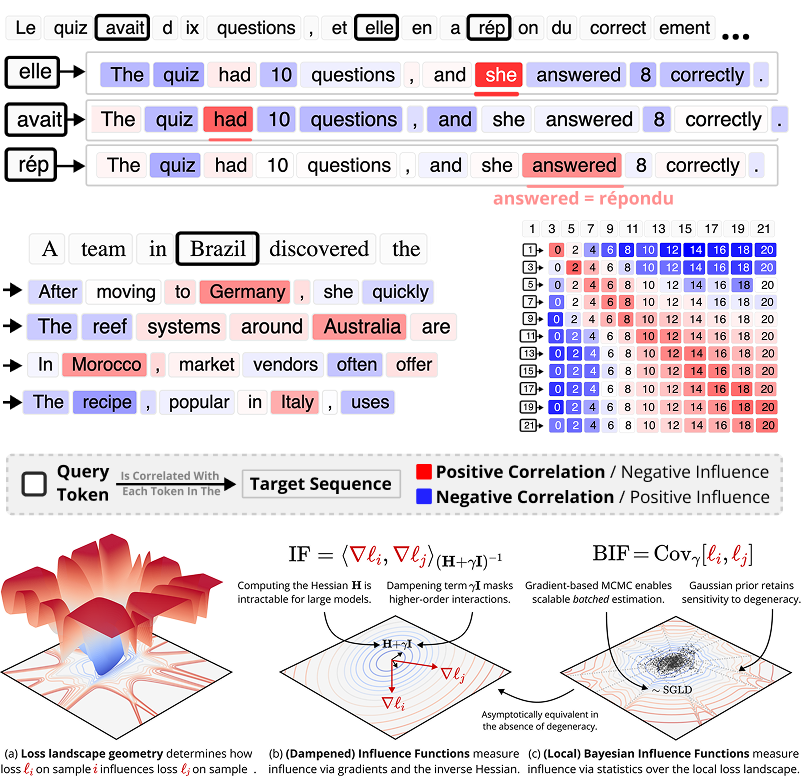
In (Kreer et al. 2025), we showed that you can scalably estimate these Bayesian influence functions using stochastic gradient MCMC techniques. The key insight is that the BIF is a covariance, and covariances can be estimated from samples. We don’t need to compute the Hessian or invert any matrix. We just need to draw samples from the local posterior and estimate sample statistics.

Concretely, we use Stochastic Gradient Langevin Dynamics (SGLD), possibly with RMSprop-style preconditioning. Starting from the checkpoint $w^*$, we continue running the optimizer but with two modifications: we add Gaussian noise at each step (to enable exploration of the posterior), and we add a “spring” term that pulls the parameters back toward $w^*$ (to keep the samples local). The update rule is:

$$w_{t+1} = w_t - \frac{\varepsilon}{2}\!\left(\frac{n\beta}{m}\sum_{k \in B_t} \nabla_w \ell_k(w_t) + \gamma(w_t - w^*)\right) + \mathcal{N}(0, \varepsilon),$$

where $\varepsilon$ is the step size, $B_t$ is a stochastic mini-batch, $\beta$ is the inverse temperature, and $\gamma$ is the precision of the localizing prior (“localization strength”). As the chain runs, we record the per-sample losses at each step, then estimate the BIF as the sample covariance across these draws (typically also across multiple chains):

$$\widehat{\text{BIF}}(z_i, z_j) = -\frac{1}{T}\sum_{t=1}^{T}\left(\ell_i(w_t) - \bar{\ell}_i\right)\left(\ell_j(w_t) - \bar{\ell}_j\right).$$

This is computationally comparable to continued training, where the memory overhead scales with the number of samples we want to attribute, not with the number of parameters. This allows the BIF to scale easily to billion-parameter models where Hessian-based methods struggle.

The hyperparameters — especially the temperature $\beta$, the localization strength $\gamma$, and the number of chains and draws — matter in a sensitive way we don’t fully understand yet. In particular, they let you capture influence at different scales of resolution.

[TODO: Cite Hugo’s upcoming work on BIF for Mechanistic Anomaly Detection.]

PauseReset0

Temperature (nβ)^-1: 0.15Localization γ: 1.00Speed: 3x

Click to place w*. The SGLD chain explores the local posterior, pulled toward w* by the localization spring (γ).

Parameters

PauseReset0

Temperature (nβ)^-1: 0.15Localization γ: 1.00Speed: 3x

Click to place w*. The SGLD chain explores the local posterior, pulled toward w* by the localization spring (γ).

Classical Influence Functions

Step 1. Assume regularity, apply the Laplace approximation, & take the large-data $n\to\infty$ limit.

Just as we Taylor expand the expected loss around a reference dataset in data space, we can Taylor expand the loss itself around a reference checkpoint $w^*$ in parameter space, i.e.:

$$\text{BIF}_{ij}(z_i, z_j) = -g_j^\top \Sigma\, g_i - \tfrac{1}{2}\text{tr}(H_j\,\Sigma\, H_i\,\Sigma) - \cdots,$$

where $g_i$ is the gradient of sample $i$ at $w^*$, $H_i$ is the associated Hessian, and $\Sigma$ is the posterior covariance.

If we assume that the posterior is regular (i.e., there is a unique minimum with a full-rank Hessian), then this expansion simplifies. Odd moments vanish, even moments factorize, and the covariance coincides with the inverse Hessian of $L(w^*)$, $\Sigma=H^{-1}(w^*)$. Truncating at leading order recovers the classical influence function,

$$\text{IF}_{ij} = -g_j^\top H(w^*)^{-1} g_i.$$

What we did is model the loss landscape as a quadratic bowl (a simple harmonic oscillator) or, equivalently, we modeled the posterior as a Gaussian (“the Laplace approximation”).

However, this regularity assumption doesn’t hold for neural networks, so the approximation is not valid. Despite its wide-spread use, the classical influence function is technically not well-defined for singular models like neural networks.

The standard “fix” is to add a damping term, replacing $H^{-1}$ with $(H + \gamma I)^{-1}$. In the BIF framework, this corresponds to using a localized posterior with $\gamma$ as the localization strength. (The damped influence function is precisely the leading-order term of the local BIF.)

But this should not be mistaken for a principled solution. Degenerate Hessian eigenvalues indicate that estimating the influence associated to those directions in parameter space requires going to higher order terms in the expansion. The damped Hessian $(H+ \gamma I)^{-1}$ models the posterior as Gaussian in all directions, including the degenerate ones, by assigning them a uniform, artificial curvature $\gamma$ rather than capturing their true (non-Gaussian) geometry.

The “classical derivation” of influence functions

If you’re familiar with influence functions, then you’ll have seen a different derivation that uses the implicit function theorem. This aside provides that alternate derivation and comments on the differences.

At a minimizer $w^*(\boldsymbol\beta)$ of $L^{\boldsymbol\beta}$, the first-order optimality condition $\nabla L^{\boldsymbol\beta}(w^*) = 0$ defines $w^*$ implicitly as a function of $\boldsymbol\beta$. Differentiating with respect to $\beta_i$:

$$\frac{dw^*}{d\beta_i} = -H^{-1}\nabla\ell_i(w^*)$$

where $H = \nabla^2 L(w^*)$ is the Hessian of the total loss. Then by the chain rule:

$$\frac{d\ell_j(w^*)}{d\beta_i} = \nabla\ell_j(w^*)^\top \frac{dw^*}{d\beta_i} = -g_j^\top H^{-1} g_i$$

This is the classical influence function. The derivation requires: (a) a unique minimum $w^*$, (b) an invertible Hessian $H$ (regularity), and (c) smooth dependence of $w^*$ on $\boldsymbol\beta$ (implicit function theorem). All three fail for neural networks, where degenerate minima are the norm, even in the underparameterized setting.

The Bayesian influence function, in contrast, makes none of these assumptions. Its main assumption is a modeling choice (that we can substitute expectations over training trajectories with expectations over a Gibbs measure). This is a mild assumption next to the assumption of regularity.

That is to say, the derivation of the classical IF as a limiting case of the BIF is no less natural than the derivation from the implicit function theorem.

Step 2. Assume a block-wise Hessian.

Most work in the TDA field focuses on approximating this damped Hessian inverse efficiently. The Hessian is a $d \times d$ matrix where $d$ is the parameter count, which ranges from millions to trillions for modern models. Storing the full Hessian requires $O(d^2)$ memory and inverting it costs $O(d^3)$ operations; both are intractable.

EK-FAC (Grosse et al. 2023) is a reference for the current state of the art. It approximates the Fisher information matrix (equivalent to the Gauss-Newton Hessian for cross-entropy loss) as a block-diagonal matrix with one block per layer, where each block is further factored as a Kronecker product of two smaller matrices: one capturing input activations, the other capturing output gradients. This reduces inversion from $O(d^3)$ to roughly $O(\sum_l d_l^{3/2})$ per layer. The trade-off is that the block-diagonal structure discards cross-layer interactions, and the Kronecker factorization is restricted to linear and convolutional layers — attention, normalization, and other modern components require separate handling or more crude approximation.

Damping λ: 1.0

Moderate damping

λ = 0: singularλ → ∞: GradSim

w* = (0.80, 0.60)

Click to place w*. The ellipse shows the Gaussian approximation to the local posterior: (H + λI)^-1.

Parameters

Damping λ: 1.0

Moderate damping

λ = 0: singularλ → ∞: GradSim

w* = (0.80, 0.60)

Click to place w*. The ellipse shows the Gaussian approximation to the local posterior: (H + λI)^-1.

Step 3. Assume a diagonal Hessian. An even simpler approximation retains only the diagonal of the Hessian, or equivalently, uses the second-moment estimates maintained by adaptive optimizers like Adam or RMSprop. This gives a per-parameter scaling of the gradients:

$$\text{DiagIF}(z_i, z_j) = -\sum_a \frac{(\nabla_a \ell_j(w^*))(\nabla_a \ell_i(w^*))}{H_{aa} + \gamma}$$

This is $O(d)$ in storage and requires no matrix operations at all. It captures the fact that different parameters operate at different scales (a real property of the loss landscape), but discards all correlations between different parameters. TrackStar (Chang et al. 2025) uses optimizer second-moment corrections in this spirit, pushing gradient-based attribution to full LLM pretraining scale.

GradSim

Step 4. Assume an isotropic landscape or take the limit of large damping.

If we additionally assume the loss landscape is isotropic (or, equivalently, take the large-$\gamma$ limit), then the Hessian inverse drops out and we discard curvature entirely, which reduces influence to a dot product between gradients:

$$\text{GradSim}(z_i, z_j) = \nabla_w \ell_j(w^*) \cdot \nabla_w \ell_i(w^*)$$

This is closely related to the empirical Neural Tangent Kernel (NTK). The NTK $\Theta(x, x') = \nabla_w f(x; w) \cdot \nabla_w f(x'; w)$ measures the similarity between inputs in terms of how the network’s output changes with respect to parameter perturbations. GradSim is the per-sample-loss analog: it measures how the loss on two samples co-varies under parameter perturbations, under the assumption that the loss landscape is locally flat. The NTK perspective makes this precise: in the infinite-width (lazy training) regime, the NTK is constant and the model is effectively linear in its parameters, which is exactly the regime where GradSim is accurate.

Step 5. Compress gradients with projections.

All of the above methods require computing and storing gradient vectors of dimension $d$. For very large models and datasets, even this is prohibitive. Random projections offer a way to reduce the cost that is orthogonal to the choice of curvature approximation: the Johnson-Lindenstrauss lemma guarantees that projecting $d$-dimensional vectors into dimension $k \ll d$ approximately preserves their inner products, and hence gradient similarities. TRAK (Park et al. 2023) applies this to GradSim; in principle, random projections can be composed with any of the above methods.

---

The Landscape of Influence

As we saw in the preceding section, a lot of current effort in the field of TDA has gone into the engineering challenge of scaling up Hessian-based influence functions to LLMs. Though this has yielded useful approximations, as a general strategy, this faces a structural issue: compute and memory costs for these methods scale superlinearly in parameter count, which means continued progress will require making ever greater sacrifices (in geometric approximations) to the gods of scaling. In addition, this focus has left certain basic theoretical challenges unaddressed.

The sampling-based approach of the BIF makes a different tradeoff. Its scaling costs are dominated by the number of samples we want to attribute, not the number of parameters. We believe this is the right tradeoff to make, because the distributional approach can go much further theoretically; it opens up three research directions that are difficult to access in the classical framework: (1) a geometric theory of influence that survives the large-data limit, (2) a natural path to higher-order interactions and connections with model internals, and (3) a connection between influence and training dynamics.

Influence as Geometry

The TDA field’s practical focus on developing new methods has obscured some foundational open questions.

One such problem is that it is unclear how to interpret influence in the modern large-data limit. For a fixed pair $(z_i, z_j)$, the BIF and its approximations scale as $O(1/n)$, so each sample’s marginal contribution to any other sample’s behavior vanishes. In the pretraining regime, where $n$ is in the billions, individual-sample influence is effectively zero.

This is a challenge for popular interpretations and applications of influence functions that view them as a tool for “explaining” which samples “are responsible” for a given observed behavior. For many behaviors of interest, vanishing influence means it may be infeasible to attribute behavior to a small number of training samples. This is further complicated by the fact that influence can change dramatically over training (discussed below). The right object may not be a sparse explanation at all, but broader structures like modes (subdistributions of the data distribution).

This does not mean that the structure of influence functions is uninformative. What survives is not the absolute magnitude of influence functions, but relative magnitudes, and we can make progress by theoretically characterizing the asymptotics. For example, in (Adam et al. 2025), we prove that the empirical BIF converges to a well-defined population quantity that we call the loss kernel:

$$K(z, z') = \lim_{\epsilon \to 0} \epsilon^{-1}\, \text{Cov}_{w \sim U(W_\epsilon)}[\ell(z; w), \ell(z'; w)]$$

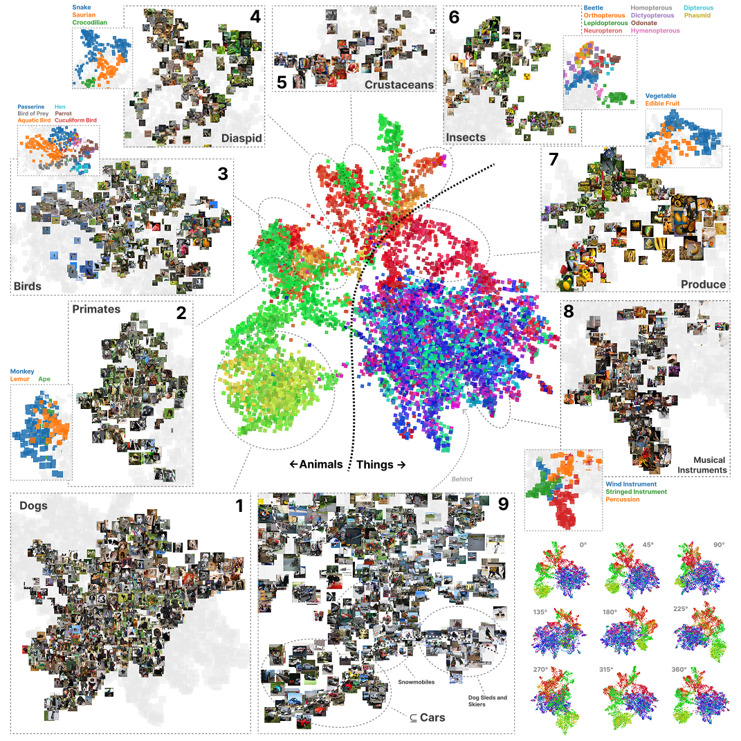
where $W_\epsilon = \{w : L(w) - L(w^*) < \epsilon\}$ is the set of near-optimal parameters. The loss kernel provides an alternative interpretation of influence as measuring functional coupling: a high value of $K(z, z')$ means that the two inputs share sensitivity to the same parameter perturbations and thus depend on the same model internals.

When combined with standard kernel analysis and visualization techniques (UMAP, clustering, kernel PCA), this connection yields new ways to map the structure the model sees in its data. Applied to Inception-v1 on ImageNet, the loss kernel reveals a hierarchical organization that mirrors the WordNet taxonomy purely from the geometry of the loss landscape, without access to labels or activations: the first split separates animate and inanimate objects, then living things by kingdom, phylum, etc. That is, influence functions are a useful tool for interpretability even if we are currently unable to use them to extract explanations.

Influence as Susceptibility

Another theoretical problem with TDA is that accurately predicting the true shape of influence may require us to go to higher-order terms in the influence expansion. Work on classical IFs begins with a regularity assumption that implicitly rules out the possibility of higher-order contributions. Thus, essentially all current work in the field focuses on just the first-order term.

Whether the influence expansion converges at all and whether it converges fast enough to admit a first-order truncation is an empirical question that has not yet been seriously interrogated. It may sometimes be appropriate; any physicist will tell you that nature is often well-behaved. But there is little reason to expect it to always suffice, especially given how singular we know loss landscapes to be (Hitchcock & Hoogland 2025).

There is another reason to care about higher-order terms besides just predictive accuracy: once influence is formulated distributionally, we can ask about the response of any observable, not just the mean loss. For example, if instead of the mean we care about the spread of sample $j$‘s loss under the local posterior, then the relevant object is the response of the variance:

$$\left.\frac{\partial}{\partial \beta_i}\operatorname{Var}_{\boldsymbol\beta}[\ell_j(w)]\right|_{\boldsymbol\beta=\mathbf 1} = -\kappa_3(\ell_i,\ell_j,\ell_j).$$

The same third cumulant that appears as the next correction to mean influence also governs how the spread of $j$‘s loss changes when we reweight sample $i$. Higher-order terms are the natural language in which to ask and answer richer response questions.

Bayesian influence functions and their higher-order counterparts are examples of susceptibilities, which is the generic term within statistical physics for “derivatives of expectation values of observables with respect to some perturbations.” The BIF is the susceptibility of the observable $\ell_j(w)$ to a perturbation in the weight of sample $i$.

Once framed this way, there are many obvious generalizations. Replace sequence-level loss with per-token loss and you obtain per-token influence functions. Replace the observable with a component-restricted loss, or with some other statistic attached to a layer, head, or circuit, and you obtain susceptibilities that begin to connect data attribution to model internals.

An inherent advantage of the sampling-based approach is that we can reuse the exact same SGLD samples to estimate susceptibilities for many different observables and at varying orders. This is because each SGLD draw implicitly aggregates contributions from all orders without ever materializing a derivative tensor.

This does not come totally for free. Higher-order moments are noisier and may require more compute (in the form of additional SGLD draws) to estimate reliably. But these costs are minor when compared with the classical Hessian-based route, where going beyond first order requires explicitly representing higher-order derivative tensors. This is prohibitive almost immediately.

In a parallel series of papers (Baker et al. 2025; Wang et al. 2025; Gordon et al. 2026), we develop a set of component-restricted susceptibilities starting with the connection between Bayesian learning and statistical physics within the frame of interpretability, rather than influence functions within the frame of influence functions. Long term, the boundary between these two is arbitrary, and the real project is developing a broader statistical physical theory of response functions in neural networks.

[TODO: Banner for Gordon et al.]

Influence as Dynamics

A last theoretical problem with classical TDA is that it assumes a static view of influence in which influence is effectively constant over training. This is a reasonable assumption for regular models, but it breaks down for singular models like neural networks that learn in distinct stages: influence measured in one stage can be completely different from influence in another.

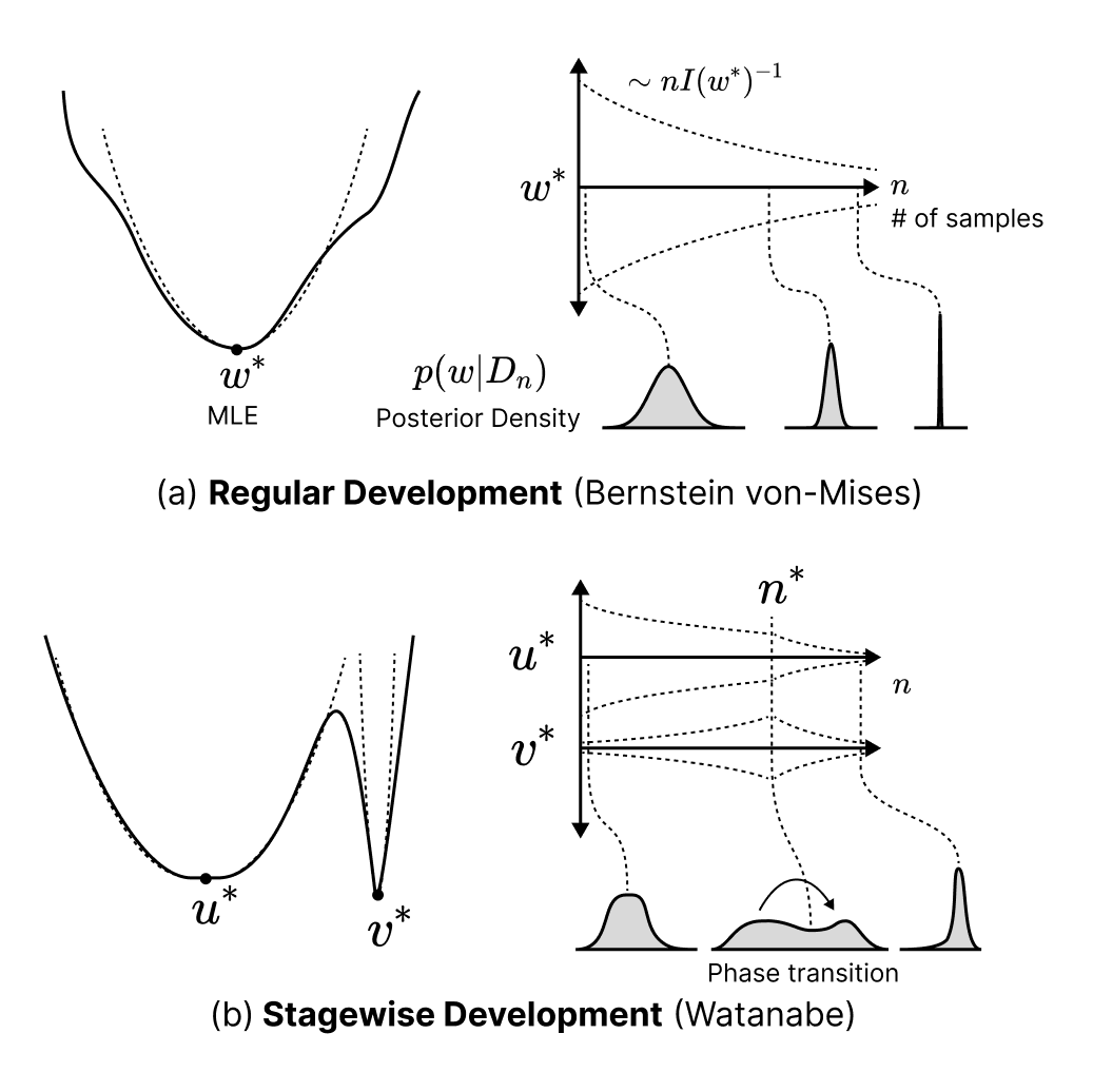
Singular learning theory predicts that it is differences in local geometry that gives rise to stagewise development. Different developmental stages (“phases”) are distinguished precisely by their different local geometries. Since the BIF depends on that local geometry, the BIF may change significantly in the phase transitions between stages.

In the previous section, we established the BIF as a susceptibility. In statistical physics, it is precisely divergences and sudden changes in susceptibilities that indicate the presence of a phase transition. This suggests using influence functions not just for data attribution but as a tool for developmental attribution to discover when something is being learned.

Viewed this way, the right goal is not to find one global influence function that is valid for all of training. The goal is to understand a sequence of local influence problems, each attached to a quasi-stable critical neighborhood, and then to stitch those local pictures together across the set of phase transitions that reorganize the model. This is the same basic strategy that appears throughout the mathematics of dynamics: in Morse theory one studies global structure by analyzing local behavior near critical points; in singularity and catastrophe theory one classifies local normal forms and then asks how global behavior changes as a system moves between them. The Developmental Interpretability agenda we have been pursuing is the corresponding local-to-global program for training dynamics.

In the case of data attribution, this program shows up in what we call stagewise data attribution. Practically, this means estimating local BIFs at a sequence of checkpoints, and asking two separate questions: what is the influence structure within each phase, and which samples or token classes dominate the between-phase spikes that mark developmental change? The aim is not only to say which data mattered, but also to say when it mattered and what local reorganization of the model it accompanied (Lee et al. 2025).

[TODO: Cite Lev’s upcoming work which shows this clearly using classical IFs.]

---

Footnotes

1. Mlodonowiecz (2025) independently advocate moving from pointwise to distributional notions of influence. ↩