Bayesian Influence Functions
Overview
A new approach to training data attribution that bypasses the Hessian inversion bottleneck and achieves state-of-the-art performance on standard benchmarks.
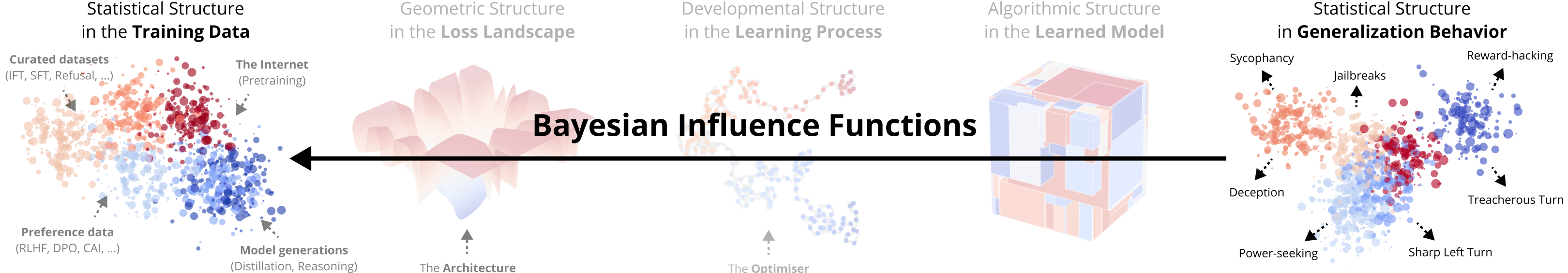
Training data attribution (TDA) studies how data influences model behavior. TDA has been recognized as relevant to many areas in technical AI safety (see Anwar et al. 2024, §2.1, 2.4, 2.6, 3.1, 3.2, etc.) and technical AI governance (see Reuel, Bucknall, et al. 2025, §3.1, 5.1). We believe this is particularly relevant to (intent) alignment.
The canonical approach to TDA is to use influence functions (IF), which estimate how much data point \(z\) affects the model's expected loss on another data point \(z'\). The problem is that standard influence functions do not work for deep neural networks; they rely on an expensive Hessian-inversion step whose memory requirements explode as models get bigger. This has spawned a line of research into influence function approximations, culminating in EK-FAC, which is the only technique we are aware of that currently scales past the 1B-parameter scale (Grosse et al. 2023).
The Bayesian influence function \(\text{BIF}(z, z')\) is a generalization of the classical IF. In a series of three papers, we introduce the local Bayesian influence function (BIF), which entirely bypasses the Hessian-inverse bottleneck. For regular models, the BIF asymptotically reduces to the classical influence function and can be seen as the expected (first-order) response to a distribution shift.
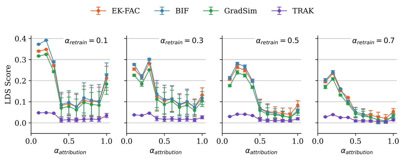
The BIF is SOTA on a standard TDA benchmark among IF-based methods in the small-dataset regime. We tested the BIF on the current standard benchmark for training data attribution: the linear datamodeling score (LDS) from the TRAK paper. The LDS measures how accurately a method predicts loss after retraining on a modified dataset. For small datasets, the BIF consistently outperforms EK-FAC (Grosse et al. 2023). For larger datasets, the BIF remains competitive in performance with baselines, though its compute costs grow faster.
This comes with several caveats: First, we believe this benchmark is contrived. Second, even if the benchmark were sensible, we still have to test the BIF across a wider range of datasets and models. Third, we don't expect that the BIF will outperform an alternative set of TDA technique known as "unrolling" methods, which involve integrating influence over the course of the training trajectory.
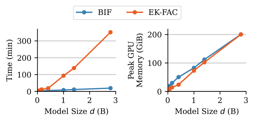
The BIF's defining advantage is its SOTA scaling with model size. The BIF bypasses the need for Hessian inversion, with memory requirements comparable to training. This makes the BIF scale far better with model size, which we validate through a comparison on the Pythia suite (see below). This comes at the cost of worse scaling with dataset size. However, the BIF compensates because it can be easily batched and parallelized, which allows us to apply the BIF for much finer-scale attribution (on a token-by-token level) compared to alternative IF-based techniques.
The BIF defines a kernel between samples. Applying dimensionality reduction to this kernel provides a way to see similarity between samples from the perspective of the model. Nearby points have similar patterns of correlation. The structure of this kernel reflects the hierarchical structure of ImageNet data. See Adam et al. (2025).
Appendices
How is the BIF related to classical influence functions?
The Classical Influence Function (CIF) and the Bayesian Influence Function (BIF) both aim to measure the effect of a single training point on a model's behavior, but they start from different theoretical foundations.
The classical influence of a training sample \(z_i\) on an observable \(\phi\) (such as the loss on a test point) is defined as the sensitivity of \(\phi\) evaluated at the optimal model parameters \(w^*\) to an infinitesimal change in the weight \(\beta_i\) of that training sample:
\[ \text{CIF}(z_i, \phi) := \frac{\partial \phi(w^*(\beta))}{\partial \beta_i}\bigg\rvert_{\beta=\mathbf{1}} \]
Here, \(w^*(\beta)\) represents the optimal parameters found by minimizing a weighted loss function,
\[ L_n(w) = \sum_{i=1}^n \beta_i \ell_i(w).\]
The CIF, therefore, relies on a single point estimate, \(w^*\), of the best model parameters.
The BIF takes a distributional approach. Instead of focusing on a single point estimate \(\phi(w^*)\), it considers the expectation of the observable over a probability distribution of possible parameters, \(\mathbb{E}_{\beta, \mathcal{D}_{\text{train}}}[\phi(w)]\). The BIF is then defined as the sensitivity of this expectation to a change in the weight of a training sample:
\[ \text{BIF}(z_i, \phi) := \frac{\partial \mathbb{E}_{\beta, \mathcal{D}_{\text{train}}}[\phi(w)]}{\partial \beta_i}\bigg\rvert_{\beta=\mathbf{1}} \]
The expectation is taken over a tempered Gibbs measure, \(p_{\beta}(w \mid \mathcal{D}_{\text{train}}) \propto \exp(-L_{\beta, \mathcal{D}_{\text{train}}}(w))\varphi(w)\), where \(\varphi(w)\) is a prior. When the loss is a negative log-likelihood, this becomes a tempered Bayesian posterior. The BIF can thus be seen as a Bayesian generalization of the classical IF, replacing a single point estimate with an average over a distribution of plausible parameters.
In particular, we introduce a local version of the BIF, which involves replacing the prior with a Gaussian centered at a reference checkpoint. This enables specializing the BIF to individual DNN checkpoints obtained through standard optimization.
For more, see Kreer et al. (2025).
How does the BIF avoid the Hessian inverse bottleneck?
The practical estimation methods for the CIF and BIF highlight their fundamental differences.
The classical approach uses the chain rule and implicit function theorem, which leads to the central formula for the CIF:
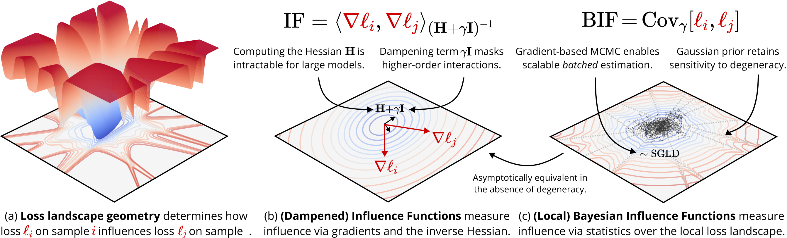
\[ \text{CIF}(z_i, \phi) = -\nabla_w \phi(w^*)^{\top} \mathbf{H}(w^*)^{-1} \nabla_{w} \ell_i(w^*) \]
where \(\mathbf{H}(w^*)\) is the Hessian matrix (the matrix of second derivatives) of the total training loss, evaluated at the optimal parameters \(w^*\). The critical step here is the inversion of the Hessian, \(\mathbf{H}^{-1}\). For modern neural networks with billions of parameters, the Hessian is a massive matrix (trillions of entries), making its computation and inversion computationally infeasible. This Hessian bottleneck is the primary obstacle to applying classical IFs to large models.
The BIF, in contrast, is estimated using an elegant formula that commonly shows up in statistical physics:
\[ \text{BIF}(z_i, \phi) = -\text{Cov}(\ell_i(w), \phi(w)) \]
This equation states that the influence of a training point is simply the negative covariance between the loss on that point, \(\ell_i(w)\), and the observable \(\phi(w)\). This covariance is computed over the posterior distribution of the weights \(w\).
The important thing is that this formula completely avoids the Hessian. Instead of an intractable matrix inversion, we have a sampling problem. We can estimate the covariance by drawing samples of the weights \(w\) from the local posterior distribution using efficient Stochastic-Gradient Markov Chain Monte Carlo (SGMCMC) techniques like SGLD, combined with a localizing prior to ensure the samples remain in a relevant region of the loss landscape. The BIF thus trades an intractable computation for a tractable sampling procedure.
For more, see Kreer et al. (2025).
What is the Linear Datamodeling Score (LDS)?
To establish a "ground truth" for data influence, an ideal experiment would be a leave-one-out retraining analysis. In this process, you would systematically remove a single data point, retrain the entire model from scratch, and measure the resulting change in performance. By repeating this for many different subsets, one could build a true map of data influence (which we can then use to benchmark influence functions and their approximations). However, for large datasets and billion-parameter models, this brute-force approach is computationally impossible, as it would require retraining a model potentially billions of times.
This practical bottleneck is what motivated the development of the Linear Datamodeling Score (LDS), introduced by the authors of TRAK. The LDS has since become a standard benchmark because it provides a scalable alternative to these leave-one-out retraining experiments.
Here's how it works:
- Subsampling: Instead of fully removing data, the benchmark creates many smaller, random subsamples of the original dataset (e.g., 100 subsamples, each containing a random 50% of the data).
- Actual Retraining: For each of these smaller subsamples, a model is retrained from a late-stage checkpoint, and the actual loss on a set of query points is recorded. This provides a cheap-to-compute, "ground truth" outcome for each subsample.
- Predicted Outcome: A TDA method, like the BIF or EK-FAC, is then asked to predict the outcome for each subsample without retraining. This prediction is a simple linear sum: the method's predicted influence for a subsample is the sum of the influences of all the individual data points included in it.
- Correlation Score: The final LDS is the Spearman's rank correlation between the list of predicted outcomes and the list of actual outcomes across the subsamples. A high score indicates that the method correctly rank which data subsamples would be most and least helpful for the model's performance.
We focused our comparison on EK-FAC because it is the current state-of-the-art influence approximation method known to scale to billion-parameter models. Our results show that the BIF is more accurate in the small-dataset regime, confirming its effectiveness on this standard benchmark.
For more, see Kreer et al. (2025).
What's wrong with the standard approach to TDA (and benchmarks like LDS)?
The standard approach to Training Data Attribution (TDA), including benchmarks like the Linear Datamodeling Score (LDS), is built on several assumptions that are invalid for modern deep neural networks. This can lead to an incomplete picture of influence. The limitations can be understood through two key aspects of the standard approach.
1. The Reliance on a Static Point Estimate
First, these methods typically study influence on a single point estimate (\(w^*\)) in parameter space. This is challenged by deep learning:
- The Problem of Degeneracy: The loss landscapes of neural networks are highly non-convex and singular. Rather than having a single, isolated minimum, the set of optimal parameters forms complex algebraic varieties where performance is equivalent. In this case, we should study the influence on the set of good solutions.
- The Role of Stochasticity: Optimizers like SGD are inherently noisy. A distributional approach, which considers a probability distribution over possible parameters, is a more natural way to model the outcome of this stochastic process.
The Bayesian Influence Function (BIF) is inherently distributional, which addresses both of these problems.
2. The Focus on a Single, Final Measurement
Second, there is an implicit assumption that a single influence measurement at the end of training provides a complete summary of a data point's role. Benchmarks like the LDS test a method's ability to predict a final, cumulative outcome, reinforcing this end-state perspective.
However, our work (Lee et al. 2025) suggests that this static view misses important parts of the learning process. A data point's influence is not a fixed quantity but a dynamic trajectory that evolves as the model develops.
- Influence is Non-Monotonic: A sample can be helpful at one stage and harmful at another.
- Timing Reveals Mechanism: The most revealing information is often contained in the dynamics of influence, such as sharp peaks or sign flips. These events often signal developmental phase transitions, where the model is acquiring a new capability. Measuring influence only at the end of training overlooks this rich, time-dependent information.
This suggests that a more complete understanding requires shifting perspective from a single, final influence score to what we term stagewise data attribution: the analysis of the full influence trajectory. This approach aims to understand not just what data had an effect, but also when and why it mattered during the model's development.
For more, see Lee et al. (2025).
How are susceptibilities (such as the BIF) related to generalization?
Susceptibilities offer a direct, quantitative link to generalization. In learning theory, generalization error is typically defined in terms of expectations of losses over distributions of data and/or parameters. The core question of out-of-distribution (OOD) generalization is understanding how these errors change when the data distribution is perturbed.
Using a Taylor series expansion, the change in generalization error can be decomposed into a series of terms: the instantaneous value, a first-order change, a second-order change, and so on. The BIF is precisely the first-order term of this expansion. It measures the linear response of the model's expected loss to an infinitesimal change in the training data distribution (specifically, the re-weighting of a single sample).
Therefore, the BIF is the fundamental tool for predicting how a model will generalize under slight distribution shifts. It provides the first correction to the in-distribution generalization error. An open empirical question is the degree of perturbation for which this linear approximation holds. Our future work will naturally involve studying the higher-order moments in this series to build an even more robust understanding of generalization.